canonical analysis in research methodology

Lesson 13: Canonical Correlation Analysis

Canonical correlation analysis explores the relationships between two multivariate sets of variables (vectors), all measured on the same individual.

Consider, as an example, variables related to exercise and health. On the one hand, you have variables associated with exercise, observations such as the climbing rate on a stair stepper, how fast you can run a certain distance, the amount of weight lifted on a bench press, the number of push-ups per minute, etc. On the other hand, you have variables that attempt to measure overall health, such as blood pressure, cholesterol levels, glucose levels, body mass index, etc.  Two types of variables are measured and the relationships between the exercise variables and the health variables are of interest.

As a second example consider variables measured on environmental health and environmental toxins. A number of environmental health variables such as frequencies of sensitive species, species diversity, total biomass, the productivity of the environment, etc. may be measured and a second set of variables on environmental toxins are measured, such as the concentrations of heavy metals, pesticides, dioxin, etc.

For a third example consider a group of sales representatives, on whom we have recorded several sales performance variables along with several measures of intellectual and creative aptitude. We may wish to explore the relationships between the sales performance variables and the aptitude variables.

One approach to studying relationships between the two sets of variables is to use canonical correlation analysis which describes the relationship between the first set of variables and the second set of variables. We do not necessarily think of one set of variables as independent and the other as dependent, though that may potentially be another approach.

• Carry out a canonical correlation analysis using SAS (Minitab does not have this functionality);
• Assess how many canonical variate pairs should be considered;
• Interpret canonical variate scores;
• Describe the relationships between variables in the first set with variables in the second set.

13.1 - Setting the Stage for Canonical Correlation Analysis

What motivates canonical correlation analysis.

It is possible to create pairwise scatter plots with variables in the first set (e.g., exercise variables), and variables in the second set (e.g., health variables). But if the dimension of the first set is p and that of the second set is q , there will be pq such scatter plots, it may be difficult, if not impossible, to look at all of these graphs together and interpret the results.

Similarly, you could compute all correlations between variables from the first set (e.g., exercise variables), and variables in the second set (e.g., health variables), however, interpretation is difficult when pq is large.

Canonical Correlation Analysis allows us to summarize the relationships into fewer statistics while preserving the main facets of the relationships. In a way, the motivation for canonical correlation is very similar to principal component analysis. It is another dimension-reduction technique.

Canonical Variates

Let's begin with the notation:

We have two variables \(X\) and \(Y\).

Suppose we have p variables in set 1: \(\textbf{X} = \left(\begin{array}{c}X_1\\X_2\\\vdots\\ X_p\end{array}\right)\)

and suppose we have q variables in set 2: \(\textbf{Y} = \left(\begin{array}{c}Y_1\\Y_2\\\vdots\\ Y_q\end{array}\right)\)

We select X and Y based on the number of variables in each set so that \(p ≤ q\). This is done for computational convenience.

We look at linear combinations of the data, similar to principal components analysis. We define a set of linear combinations named U and V . U corresponds to the linear combinations from the first set of variables, X , and V corresponds to the second set of variables, Y . Each member of U is paired with a member of V . For example, \(U_{1}\) below is a linear combination of the p X variables and \(V_{1}\) is the corresponding linear combination of the q Y variables. Similarly, \(U_{2}\) is a linear combination of the p X variables, and \(V_{2}\) is the corresponding linear combination of the q Y variables. And, so on...

\begin{align} U_1 & =  a_{11}X_1 + a_{12}X_2 + \dots + a_{1p}X_p \\ U_2 & =  a_{21}X_1 + a_{22}X_2 + \dots + a_{2p}X_p \\ &  \vdots \\ U_p & =  a_{p1}X_1 +a_{p2}X_2 + \dots +a_{pp}X_p\\ &  \\ V_1 & =  b_{11}Y_1 + b_{12}Y_2 + \dots + b_{1q}Y_q \\ V_2 & =  b_{21}Y_1 + b_{22}Y_2 + \dots +b_{2q}Y_q \\ &  \vdots \\ V_p & =  b_{p1}Y_1 +b_{p2}Y_2 + \dots +b_{pq}Y_q\end{align}

Thus define

\((U_i, V_i)\)

as the \(i^{th}\) canonical variate pair . ( \(U_{1}\), \(V_{1}\)) is the first canonical variate pair, similarly ( \(U_{2}\), \(V_{2}\)) would be the second canonical variate pair, and so on. With \(p ≤ q\) there are p canonical covariate pairs.

We hope to find linear combinations that maximize the correlations between the members of each canonical variate pair.

We compute the variance of \(U_{i}\) variables with the following expression:

\(\text{var}(U_i) = \sum\limits_{k=1}^{p}\sum\limits_{l=1}^{p}a_{ik}a_{il}cov(X_k, X_l)\)

The coefficients \(a^{i1}\) through \(a^{ip}\) that appear in the double sum are the same coefficients that appear in the definition of \(U_{i}\). The covariances between the \(k^{th}\) and \(l^{th}\) X -variables are multiplied by the corresponding coefficients \(a^{ik}\) and \(a^{il}\) for the variate \(U_{i}\).

Similar calculations can be made for the variance of \(V_{j}\) as shown below:

\(\text{var}(V_j) = \sum\limits_{k=1}^{p} \sum\limits_{l=1}^{q} b_{jk}b_{jl}\text{cov}(Y_k, Y_l)\)

The covariance between \(U_{i}\) and \(V_{j}\) is:

\(\text{cov}(U_i, V_j) = \sum\limits_{k=1}^{p} \sum\limits_{l=1}^{q}a_{ik}b_{jl}\text{cov}(X_k, Y_l)\)

The correlation between \(U_{i}\) and \(V_{j}\) is calculated using the usual formula. We take the covariance between the two variables and divide it by the square root of the product of the variances:

\(\dfrac{\text{cov}(U_i, V_j)}{\sqrt{\text{var}(U_i) \text{var}(V_j)}}\)

The canonical correlation is a specific type of correlation. The canonical correlation for the \(i^{th}\) canonical variate pair is simply the correlation between \(U_{i}\) and \(V_{i}\):

\(\rho^*_i = \dfrac{\text{cov}(U_i, V_i)}{\sqrt{\text{var}(U_i) \text{var}(V_i)}} \)

This is the quantity to maximize. We want to find linear combinations of the X 's and linear combinations of the Y 's that maximize the above correlation.

Canonical Variates Defined

Let us look at each of the p canonical variates pair individually.

First canonical variate pair: \( \left( U _ { 1 } , V _ { 1 } \right)\):

The coefficients \(a_{11}, a_{12}, \dots, a_{1p}\) and \(b_{11}, b_{12}, \dots, b_{1q}\) are selected to maximize the canonical correlation \(\rho^*_1\) of the first canonical variate pair. This is subject to the constraint that variances of the two canonical variates in that pair are equal to one.

\(\text{var}(U_1) = \text{var}(V_1) = 1\)

This is required to obtain unique values for the coefficients.

Second canonical variate pair: \( \left( U _ { 2 } , V _ { 2 } \right)\)

Similarly we want to find the coefficients \(a_{21}, a_{22}, \dots, a_{2p}\) and \(b_{21}, b_{22}, \dots, b_{2q}\) that maximize the canonical correlation \(\rho^*_2\) of the second canonical variate pair, \( \left( U _ { 2 } , V _ { 2 } \right)\).  Again, we will maximize this canonical correlation subject to the constraint that the variances of the individual canonical variates are both equal to one.  Furthermore, we require the additional constraints that \( \left( U _ { 1 } , U _ { 2 } \right)\), and \( \left( V_{1} ,  V_{2} \right)\) are uncorrelated.  In addition, the combinations \( \left( U_{1} ,  V_{2} \right)\) and \( \left( U_{2} , V_{1} \right)\) must be uncorrelated. In summary, our constraints are:

\(\text{var}(U_2) = \text{var}(V_2) = 1\),

\(\text{cov}(U_1, U_2) = \text{cov}(V_1, V_2) = 0\),

\(\text{cov}(U_1, V_2) = \text{cov}(U_2, V_1) = 0\).

Basically, we require that all of the remaining correlations equal zero.

This procedure is repeated for each pair of canonical variates. In general, ...

\( i^{th} \) canonical variate pair: \( \left( U _ { i } , V _ { i } \right)\)

We want to find the coefficients \(a_{i1}, a_{i2}, \dots, a_{ip}\) and \(b_{i1}, b_{i2}, \dots, b_{iq}\) that maximize the canonical correlation \(\rho^*_i\) subject to the constraints that

\(\text{var}(U_i) = \text{var}(V_i) = 1\),

\(\text{cov}(U_1, U_i) = \text{cov}(V_1, V_i) = 0\),

\(\text{cov}(U_2, U_i) = \text{cov}(V_2, V_i) = 0\),

\(\text{cov}(U_{i-1}, U_i) = \text{cov}(V_{i-1}, V_i) = 0\),

\(\text{cov}(U_1, V_i) = \text{cov}(U_i, V_1) = 0\),

\(\text{cov}(U_2, V_i) = \text{cov}(U_i, V_2) = 0\),

\(\text{cov}(U_{i-1}, V_i) = \text{cov}(U_i, V_{i-1}) = 0\).

Again, requiring all of the remaining correlations to be equal to zero.

Next, let's see how this is carried out in SAS...

13.2 - Example: Sales Data

Example 13-1: sales.

The example data comes from a firm that surveyed a random sample of n = 50 of its employees in an attempt to determine which factors influence sales performance. Two collections of variables were measured:

• Sales Growth
• Sales Profitability
• New Account Sales
• Mechanical Reasoning
• Abstract Reasoning
• Mathematics

There are p = 3 variables in the first group relating to Sales Performance and q  = 4 variables in the second group relating to Test Scores.

Download the text file containing the data here: sales.csv

•   Example

Canonical Correlation Analysis is carried out in SAS using a canonical correlation procedure that is abbreviated as cancorr . Let's look at how this is carried out in the SAS Program below

Download the SAS program here: sales.sas or click on the copy icon inside Explore the Code.

Note : In the upper right-hand corner of the code block you will have the option of copying (   ) the code to your clipboard or downloading (   ) the file to your computer.

13.3. Test for Relationship Between Canonical Variate Pairs

Let's first determine if there is any relationship between the two sets of variables at all. Perhaps the two sets of variables are completely unrelated to one another and independent!

To test for independence between the Sales Performance and the Test Score variables, first, consider a multivariate multiple regression model where we predict the Sales Performance variables from the Test Score variables.  In this general case, we have p multiple regressions, each multiple regression predicting one of the variables in the first group ( X variables) from the q variables in the second group ( Y variables).

\begin{align} X_1 & =  \beta_{10} + \beta_{11}Y_1 +\beta_{12}Y_2 + \dots +\beta_{1q}Y_q + \epsilon_1 \\ X_2 & =  \beta_{20}+ \beta_{21}Y_1 + \beta_{22}Y_2 + \dots +\beta_{2q}Y_q + \epsilon_2 \\  &  \vdots \\ X_p & =  \beta_{p0} + \beta_{p1}Y_1 + \beta_{p2}Y_2 + \dots + \beta_{pq}Y_q + \epsilon_p \end{align}

In our example, we have multiple regressions predicting the p = 3 sales variables from the q = 4 test score variables. We wish to test the null hypothesis that these regression coefficients (except for the intercepts) are all equal to zero. This would be equivalent to the null hypothesis that the first set of variables is independent of the second set of variables.

\(H_0\colon \beta_{ij} = 0;\)  \( i = 1,2, \dots, p; j = 1,2, \dots, q\)

This is carried out using Wilks lambda. The results of this are found on page 1 of the output of the SAS Program.

Test of H0: The canonical correlations in the current row and all that follow are zero

SAS reports Wilks lambda \(\Lambda = 0.00215 ; F = 87.39 ; d . f = 12,114 ; p < 0.0001\). Wilks lambda is a ratio of two variance-covariance matrices (raised to a certain power).  If the values of these statistics are large (small p -value), then we reject the null hypothesis.  In our example, we reject the null hypothesis that there is no relationship between the two sets of variables and conclude that the two sets of variables are dependent. Note also that the above null hypothesis is also equivalent to testing the null hypothesis that all p canonical variate pairs are uncorrelated, or

\(H_0\colon \rho^*_1 = \rho^*_2 = \dots = \rho^*_p = 0 \)

Because Wilks lambda is significant and the canonical correlations are ordered from largest to smallest, we can conclude that at least \(\rho^*_1 \ne 0\).

We may also wish to test the hypothesis that the second or the third canonical variate pairs are correlated. We can do this in successive tests. Next, test whether the second and third canonical variate pairs are correlated...

\(H_0\colon \rho^*_2 = \rho^*_3 = 0\)

We can look again at the SAS output above. In the second row for the likelihood ratio test statistic we find \(L ^ { \prime } = 0.19524 ; F = 18.53 ; d . f = 6,88 ; p < 0.0001\) . From this test we can conclude that the second canonical variate pair is correlated, \(\rho^*_2 \ne 0\).

Finally, we can test the significance of the third canonical variate pair.

\(H_0\colon \rho^*_3 = 0\)

The third row of the SAS output contains the likelihood ratio test statistic \(L ^ { \prime } = 0.8528 ; F = 3.88 ; d . f = 2,45 ; p = 0.0278\) . This is also significant and so we conclude that the third canonical variate pair is correlated.

All three canonical variate pairs are significantly correlated and dependent on one another. This suggests that we may summarize all three pairs. In practice, these tests are carried out successively until you find a non-significant result. Once a non-significant result is found, you stop. If this happens with the first canonical variate pair, then there is not sufficient evidence of any relationship between the two sets of variables and the analysis may stop.

If the first pair shows significance, then you move on to the second canonical variate pair. If this second pair is not significantly correlated then stop. If it was significant you would continue to the third pair, proceeding in this iterative manner through the pairs of canonical variates testing until you find non-significant results.

13.4 - Obtain Estimates of Canonical Correlation

Now that we rejected the hypotheses of independence, the next step is to obtain estimates of canonical correlation.

The estimated canonical correlations are found at the top of page 1 in the SAS output as shown below:

Canonical Correlation Analysis

The squared values of the canonical variate pairs, found in the last column, can be interpreted much in the same way as \(r^{2}\) values are interpreted.

We see that 98.9% of the variation in \(U_{1}\) is explained by the variation in \(V_{1}\), and 77.11% of the variation in \(U_{2}\) is explained by \(V_{2}\), but only 14.72% of the variation in \(U_{3}\) is explained by \(V_{3}\). These first two are very high canonical correlations and suggest that only the first two canonical correlations are important.

One can actually see this from the plots that SAS generates.  The first canonical variate for sales is plotted against the first canonical variate for scores in the scatter plot for the first canonical variate pair:

Canonical Correlation Analysis - Sales Data

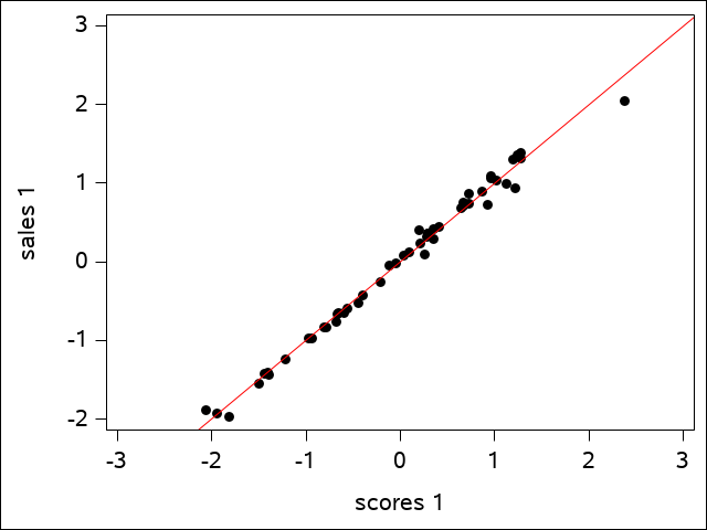
The regression line shows how well the data fits. The plot of the second canonical variate pair is a bit more scattered, but is still a reasonably good fit:

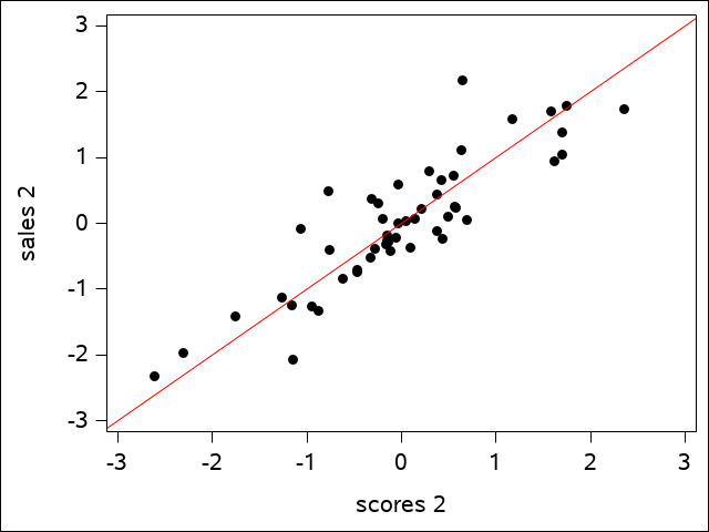
A plot of the third pair would show little of the same kind of fit.  We may refer to only the first two canonical variate pairs from this point on based on the observation that the third squared canonical correlation value is so small.

13.5 - Obtain the Canonical Coefficients

Page 2 of the SAS output provides the estimated canonical coefficients \(\left(a_{ij}\right)\) for the sales variables:

Raw Canonical Coefficients for the Sales Variables

Using the coefficient values in the first column, the first canonical variable for sales is determined using the following formula:

\(U_1 = 0.0624X_{growth}+0.0209X_{profit}+0.0783X_{new}\)

Likewise, the estimated canonical coefficients \(\left(b_{ij}\right)\) for the test scores are located in the next table in the SAS output:

Raw Canonical Coefficients for the Test Scores

Using the coefficient values in the first column, the first canonical variable for test scores is determined using a similar formula:

\(V_1 = 0.0697Y_{create}+0.0307Y_{mech}+0.0896Y_{abstract}+0.0628Y_{math}\)

In both cases, the magnitudes of the coefficients give the contributions of the individual variables to the corresponding canonical variable. However, just like in principal components analysis, these magnitudes also depend on the variances of the corresponding variables. Unlike principal components analysis, however, standardizing the data has no impact on the canonical correlations.

13.6 - Interpret Each Component

To interpret each component, we must compute the correlations between each variable and the corresponding canonical variate.

The correlations between the sales variables and the canonical variables for Sales Performance are found at the top of the fourth page of the SAS output in the following table:

Correlations Between the Sales Variables and Their Canonical Variables

Looking at the first canonical variable for sales, we see that all correlations are uniformly large. Therefore, you can think of this canonical variate as an overall measure of Sales Performance. For the second canonical variable for Sales Performance, none of the correlations are particularly large, and so, this canonical variable yields little information about the data. Again, we had decided earlier not to look at the third canonical variate pairs.

A similar interpretation can take place with the Test Scores.

b. The correlations between the test scores and the canonical variables for Test Scores are also found in the SAS output:

Correlations Between the Test Scores and Their Canonical Variables

Because all correlations are large for the first canonical variable, this can be thought of as an overall measure of test performance as well, however, it is most strongly correlated with mathematics test scores. Most of the correlations with the second canonical variable are small. There is some suggestion that this variable may be negatively correlated with abstract reasoning.

c. Putting (a) and (b) together, we see that the best predictor of sales performance is mathematics test scores as this indicator stands out the most.

13.7 - Reinforcing the Results

These results are further reinforced by looking at the correlations between each set of variables and the opposite group of canonical variates.

Correlations Between the Sales Variables and the Canonical Variables of the Test Scores

We can see that all three of these correlations are strong and show a pattern similar to that with the canonical variate for sales. The reason for this is obvious: The first canonical correlation is very high.

The correlations between the test scores and the first canonical variate for sales are also in the SAS output:

Correlations Between the Test Scores and the Canonical Variables of the Sales Variables

These results confirm that sales performance is best predicted by mathematics test scores.

13.8 - Summary

In this lesson we learned about:

• How to test for independence between two sets of variables
• How to determine the number of significant canonical variate pairs
• How to compute the canonical variates from the data
• How to interpret each member of a canonical variate pair using its correlations with the member variables
• How to use the results of canonical correlation analysis to describe the relationships between two sets of variables

An official website of the United States government

The .gov means it’s official. Federal government websites often end in .gov or .mil. Before sharing sensitive information, make sure you’re on a federal government site.

The site is secure. The https:// ensures that you are connecting to the official website and that any information you provide is encrypted and transmitted securely.

• Publications
• Account settings

Preview improvements coming to the PMC website in October 2024. Learn More or Try it out now .

• Advanced Search
• Journal List
• Hum Brain Mapp
• v.41(13); 2020 Sep

A technical review of canonical correlation analysis for neuroscience applications

Xiaowei zhuang.

1 Cleveland Clinic Lou Ruvo Center for Brain Health, Las Vegas Nevada, USA

Zhengshi Yang

Dietmar cordes.

2 University of Colorado, Boulder Colorado, USA

3 Department of Brain Health, University of Nevada, Las Vegas Nevada, USA

Associated Data

There is no data or code involved in this review article.

Collecting comprehensive data sets of the same subject has become a standard in neuroscience research and uncovering multivariate relationships among collected data sets have gained significant attentions in recent years. Canonical correlation analysis (CCA) is one of the powerful multivariate tools to jointly investigate relationships among multiple data sets, which can uncover disease or environmental effects in various modalities simultaneously and characterize changes during development, aging, and disease progressions comprehensively. In the past 10 years, despite an increasing number of studies have utilized CCA in multivariate analysis, simple conventional CCA dominates these applications. Multiple CCA‐variant techniques have been proposed to improve the model performance; however, the complicated multivariate formulations and not well‐known capabilities have delayed their wide applications. Therefore, in this study, a comprehensive review of CCA and its variant techniques is provided. Detailed technical formulation with analytical and numerical solutions, current applications in neuroscience research, and advantages and limitations of each CCA‐related technique are discussed. Finally, a general guideline in how to select the most appropriate CCA‐related technique based on the properties of available data sets and particularly targeted neuroscience questions is provided.

Neuroscience applications of canonical correlation analysis (CCA) and its variants are systematically reviewed from a technical perspective. Detailed formulations, analytical and numerical solutions, current applications, and advantages and limitations of CCA and its variants are discussed. A general guideline to select the most appropriate CCA‐related technique is provided.

1. INTRODUCTION

Recently in neuroscience research, multiple types of data are usually collected from the same individual, including demographics, clinical symptoms, behavioral and neuropsychological measures, genetic information, structural and functional magnetic resonance imaging (fMRI) data, position emission tomography (PET) data, functional near‐infrared spectroscopy (fNIRS) data, and electrophysiological data. Each of these data types, termed modality here, contains multiple measurements and provides a unique view of the subject. These measurements can be the raw data (e.g., neuropsychological tests) or derived information (e.g., brain regional volume and thickness measures derived from T1‐weighted MRI).

Neuroscience research has been focused on uncovering associations between measurements from multiple modalities. Conventionally, a single measurement is selected from each modality, and their one‐to‐one univariate association is analyzed. Multiple correction is then performed to guarantee statistically meaningful results. These univariate associations have illuminated numerous findings in various neurological diseases, such as association between gray‐matter density and Mini Mental State Examination score in Alzheimer's disease (Baxter et al., 2006 ), correlation between brain network temporal dynamics and Unified Parkinson Disease Rating Scale part III motor scores in Parkinson's disease subjects (Zhuang et al., 2018 ), and relationship between imaging biomarkers and cognitive performances in fighters with repetitive head trauma (Mishra et al., 2017 ).

However, the one‐to‐one univariate association overlooks the multivariate joint relationship among multiple measurements between modalities. Furthermore, when dealing with brain imaging data, highly correlated noise further decreases the effectiveness and sensitivity of mass‐univariate voxel‐wise analysis (Cremers, Wager, & Yarkoni, 2017 ; Zhuang et al., 2017 ), and different methods of multiple corrections might lead to various statistically meaningful results. Multivariate analysis, alternatively, uncovers the joint covariate patterns among different modalities and avoids multiple correction steps, which would be more appropriate to disentangle joint relationship between modalities and guarantees full utilization of all common information.

Canonical correlation analysis (CCA) is one candidate to uncover these joint multivariate relationships among different modalities. CCA is a statistical method that finds linear combinations of two random variables so that the correlation between the combined variables is maximized (Hotelling, 1936 ). CCA can identify the source of common statistical variations among multiple modalities, without assuming any particular form of directionality, which suits neuroscience applications. In practice, CCA has been mainly implemented as a substitute for univariate general linear model (GLM) to link different modalities, and therefore, is a major and powerful tool in multimodal data fusion. Multiple CCA variants, including kernel CCA, constrained CCA, deep CCA, and multiset CCA, also have been applied in neuroscience research. However, the complicated multivariate formulations and obscure capabilities remain obstacles for CCA and its variants to being widely applied.

In this study, we review CCA applications in neuroscience research from a technical perspective to improve the understanding of the CCA technique itself and to provide neuroscience researchers with guidlines of proper CCA applications. We briefly discuss studies through December 2019 that have utilized CCA and its variants to uncover the association between multiple modalities. We explain the existing CCA method and its variants for their formulations, properties, relationships to other multivariate techniques, and advantages and limitations in neuroscience applications. We finally provide a flowchart and an experimental example to assist researchers to select the most appropriate CCA technique based on their specific applications.

2. INCLUSION/EXCLUSION OF STUDIES

Using the PubMed search engine in December 2019, we searched neuroimaging or neuroscience articles using CCA with the following string: (“canonical correlation” analysis) AND (neuroscience OR neuroimaging). This search yielded 192 articles; 11 additional articles were included based on authors' preidentification. We excluded non‐English articles, conference abstracts and duplicated studies, yielding 188 articles assessed for eligibility. We further identified 160 studies that met the following criteria: (a) primarily focused on a CCA or CCA‐variant technique and (b) with an application to neuroimaging or neuroscience modalities. Reasons for exclusion and numbers of articles meeting exclusion criteria at each stage are shown in Figure ​ Figure1 1 .

Inclusion and exclusion criteria for this review

The remaining articles were full‐text reviewed and divided into five categories based on the applied CCA technique (Figure ​ (Figure2a): 2a ): CCA ( N = 67); constrained CCA ( N = 53); nonlinear CCA ( N = 7); multiset CCA ( N = 29); and CCA‐other ( N = 7). Three articles applied constrained multiset CCA, thus are categorized into both constrained CCA and multiset CCA. Numbers of articles of every year from 1990 to 2019 are plotted in Figure ​ Figure2 2 (B).

Number of articles summarized by category (a) and year (b)

In the following sections, we present technical details (Section 3 ) and neuroscience applications for each category (Section 4 ). In Section 5 , we discuss technical differences and summarize advantages and limitations of each CCA‐related technique. We finally provide an experimental example and guidance in Section 6 to researchers who are interested in applying multivariate CCA‐related techniques in their work.

3. TECHNICAL DETAILS

Figure ​ Figure3 3 shows the detailed CCA equations (red box) and linkages between CCA and its variants. Constrained CCA (yellow boxes), nonlinear CCA (gray boxes), and multiset CCA (orange boxes) are focused, and linkages between CCA and other univariate (light green boxes) and multivariate (dark green boxes) techniques are also included. Here, we provide basic formulations and solutions of each CCA and its variants. We also discuss how CCA is mathematically linked to its variants and to other multivariate or univariate techniques. Researchers interested in further details can refer to the corresponding references.

Technical details of CCA and relationship between CCA and its variants. Background color indicates different techniques: red: conventional CCA; gray: nonlinear CCA; yellow: constrained CCA; orange: multiset CCA; green: other techniques related to CCA. CCA, canonical correlation analysis; PCA, principle component analysis; PLS, partial least square

3.1. Conventional CCA

Formulations.

CCA is designed to maximize the correlation between two latent variables y 1 ∈ R p 1 × 1 and y 2 ∈ R p 2 × 1 , which are also being referred to as modalities. Here, we denote Y k ∈ R N × p k , k = 1 , 2 as collected samples of these two variables, where N represents the number of observations (samples) and p k , k = 1, 2 represent the number of features in each variable. CCA determines the canonical coefficients u 1 ∈ R p 1 × 1 and u 2 ∈ R p 2 × 1 for Y 1 and Y 2 , respectively, by maximizing the correlation between Y 1 u 1 and Y 2 u 2 :

In Equation (1 ), ∑ 11 and ∑ 22 are the within‐set covariance matrices and ∑ 12 is the between‐set covariance matrix. The denominator in Equation (1 ) is used to normalize within‐set covariance, which guarantees that CCA is invariant to the scaling of coefficients.

Canonical coefficients u 1 and u 2 can be found by setting the partial derivative of the objective function (Equation (1 )) with respect to u 1 and u 2 to zero, respectively, leading to:

Equation (2 ) can be further reduced to a classical eigenvalue problem, if ∑ kk is invertible, as follows:

Each pair of canonical coefficients { u 1 ,  u 2 } are the eigenvectors of ∑ 11 − 1 ∑ 12 ∑ 22 − 1 ∑ 21 and ∑ 22 − 1 ∑ 21 ∑ 11 − 1 ∑ 12 , respectively with the same eigenvalue ρ 2 . Following Equation (3 ), up to M = min( p 1 ,  p 2 ) pairs of canonical coefficients can be achieved through singular value decomposition (SVD), and every pair of canonical variables Y 1 u 1 m Y 2 u 2 m , m = 1 , 2 , … , M , are uncorrelated with another pair of canonical variables. Corresponding M canonical correlation values are in descending order as ρ (1)  >  ρ (2)  > … >  ρ ( M ) .

As we stated above, one requirement for solving the CCA problem (Equation (1 )) through this eigenvalue problem (Equation (3 )) is that within‐set covariance matrices ∑ 11 and ∑ 22 must be invertible. To satisfy this requirement, the number of observations in Y 1 and Y 2 should be greater than the number of features, that is, N  >  p k , k = 1, 2. Furthermore, since the square of canonical correlation values ( ρ 2 ) are the eigenvalues of matrices ∑ 11 − 1 ∑ 12 ∑ 22 − 1 ∑ 21 and ∑ 22 − 1 ∑ 21 ∑ 11 − 1 ∑ 12 , both matrices are required to be positive definite.

Statistical inferences

Parametric inferences exist for CCA if both variables strictly follow the Gaussian distribution. The null hypothesis is that no (zero) canonical correlation exists between Y 1 and Y 2 , that is, ρ (1) = ρ (2) = … = ρ ( M ) = 0. The alternative hypothesis is that at least one canonical correlation value is nonzero. A test statistic based on Wilk's Λ is (Bartlett, 1939 ):

which follows a chi‐square distribution χ p 1 × p 2 2 with degree of freedom of p 1  ×  p 2 . It is also of interest to test if a specific canonical correlation value ( ρ ( m ) , 1 ≤  m  ≤  M ) is different from zero. In this case, the test statistic in Equation (4 ) becomes:

which follows χ p 1 − m p 2 − m 2 .

In practice, this parametric inference is not commonly used since it requires variables to strictly follow the Gaussian distribution and is sensitive to outliers (Bartlett, 1939 ). Instead, permutation‐based nonparametric statistics have been widely used in CCA applications. In general, observations of one variable are randomly shuffled ( Y 1 becomes Y 1 ^ ) while observations of the other variable are kept intact ( Y 2 remains). A new set of canonical correlation values are then computed for Y 1 ^ and Y 2 following Equation (3 ). This random shuffling is repeated multiple times, and the null distribution of canonical correlation values is generated. Statistical significance ( p ‐values) for the true canonical correlation values are finally obtained from this null distribution.

3.2. CCA variants

The conventional CCA (Equation (1 )) can be modified for different purposes. Constrained CCA penalizes canonical coefficients u 1 and u 2 to satisfy certain requirements and more specifically, to avoid overfitting and unstable results caused by insufficient observations in Y 1 or Y 2 . Kernel and deep CCA are designed to uncover nonlinear correlations between modalities by projecting the original variables to new nonlinear feature spaces. Multiset CCA is proposed to find multivariate associations among more than two modalities. In this section, we systematically review constrained CCA, nonlinear CCA, multiset CCA, and other special CCA cases.

3.2.1. Constrained CCA

Generalized constrained cca, formulation.

Constrained CCA is implemented by adding penalties to coefficients u k in Equation (1 ). Penalties can be either equality constraints or inequality constraints, and based on researcher's own considerations, penalties can be added to either u 1 or u 2 , or to both u 1 and u 2 . Therefore, in general, the constrained CCA problem can be formulated in terms of the constrained optimization problem as:

where E represents the set of equality constraints and InE represents the set of inequality constraints.

Analytical solutions usually do not exist for constrained CCA problems, and solving Equation (6 ) requires numerical solutions through iterative optimization techniques. Multiple optimization techniques can be applied, such as the Broyden–Fletcher–Goldfarb–Shanno algorithm, augmented‐Lagrangian algorithm, reduced gradient method and sequential quadratic programming. Examples and details of solving constrained CCA problems through above optimization techniques can be found in Yang, Zhuang, et al. ( 2018 ) and Zhuang et al. ( 2017 ).

Special case: L 1 ‐norm penalty and sparse CCA

The most commonly implemented penalty in constrained CCA is the L 1 ‐norm penalty added to either u 1 or u 2 , and is termed sparse CCA:

where | u i | 1  <  c i are inequality constraints.

The L 1 ‐norm penalty induces sparsity on canonical coefficients, and therefore sparse CCA can be implemented to high‐dimensional variables. When dealing with high‐dimensional variables, the within‐set covariance matrices ∑ 11 and ∑ 22 in Equation (7 ) are also high‐dimensional matrices, which are memory intensive. In addition, when the number of observations is less than the number of features, the covariance matrices cannot be estimated reliably from the sample. In these cases, within‐set covariance matrices are usually replaced by identity matrices, and sparse CCA is then equivalent to sparse PLS. Please note that researchers may still name this technique as sparse CCA even after this replacement (Witten, Tibshirani, & Hastie, 2009 ).

With known prior information about features or observations, sparse CCA can be further modified to structure sparse CCA or discriminant sparse CCA , respectively. If the known prior information is about features, such as categorizing features into different groups (Lin et al., 2014 ) or characterizing connections between features (Kim et al., 2019 ), the prior information will be implemented as an additional penalty on features, leading to structure sparse CCA . Alternatively, if the known prior information is about observations, such as diagnostic group of each subject, the prior information will be implemented as additional constraint on observations, leading to discriminant sparse CCA (Wang et al., 2019 ).

Sparse CCA, structure sparse CCA, and discriminant sparse CCA can all be considered as special cases of a generalized constrained CCA (Equation (6 )) problem with different equality and inequality constraint sets. Iterative optimization techniques used to solve the generalized constrained CCA problem are also applicable here to solve these special cases.

3.2.2. Nonlinear CCA

Both CCA and constrained CCA assume linear intervariable relationships, however, this assumption does not hold in general for all variables in real data. Nonlinear CCA uncovers the joint nonlinear relationship between different variables, which is a complementary tool to conventional CCA methods. Kernel CCA, temporal kernel CCA, and deep CCA are the foremost techniques in this category.

Kernel CCA and temporal kernel CCA

Kernel CCA uncovers the joint nonlinear relationship between two variables by mapping the original feature space in Y 1 and Y 2 on to a new feature space through a predefined kernel function . However, this new feature space is not explicitly defined. Instead, the original feature space for each observation in Y k is implicitly projected to a higher dimensional feature space Y k  →  ϕ ( Y k ) embedded in a prespecified kernel function H k ∈ R N × N , which is independent of the number of features in the projected space. After transforming u k to ϕ ( Y k ) T v k , the CCA form in Equation (1 ) in the higher dimensional feature space, namely kernel CCA can be written as:

where v 1 and v 2 are unknowns to estimate, instead of u 1 and u 2 .

Temporal kernel CCA is a kernel CCA variant that is specifically designed for two time series with temporal delays. In temporal kernel CCA, one variable, for example, Y 1 , is shifted for multiple different time points and a new variable Y ~ 1 is formed by concatenating the original Y 1 and the temporally shifted Y 1 . The new variable Y ~ 1 and the original Y 2 are then input to kernel CCA as in Equation (8 ).

Closed‐form analytical solution exists for kernel CCA (Equation (8 )). By setting the partial derivatives of the objective function in Equation (8 ) with respect to v 1 and v 2 to zero separately, kernel CCA can be converted to the following problem:

Note that the kernel CCA problem defined in Equation (9 ) always holds true when ρ = 1. To avoid this trivial solution, a penalty term needs to be introduced to the norm of original canonical coefficients u k , such that v k T H k 2 v k become v k T H k 2 v k + λ u k 2 = v k T H k 2 + λ H k v k , where λ is a regularization parameter. This regularized kernel CCA problem can be further represented as an eigenvalue problem (Hardoon, Szedmak, & Shawe‐Taylor, 2004 ):

where a closed‐form solution exists in the new feature space.

Kernel CCA requires a predefined kernel function for the feature mapping to uncover the joint nonlinear relationship between two variables. Alternatively, recent development of deep learning makes it possible to learn the feature mapping from data itself. The deep learning variant of CCA, deep CCA (Andrew, Bilmes, & Livescu, 2013 ), provides a more flexible and robust way to learn and search the nonlinear association between two variables. More specifically, deep CCA first passes the original Y 1 and Y 2 through multiple stacked layers of nonlinear transformations. Let θ 1 and θ 2 represent vectors of all parameters through all layers for Y 1 and Y 2 , respectively, deep CCA can be represented as:

Deep CCA is solved through a deep learning schema by dividing the original data into training and testing sets. θ 1 and θ 2 are optimized by following the gradient of the correlation objective as estimated on the training data (Andrew et al., 2013 ). The number of unknown parameters in deep CCA is much higher than the number of unknowns in other CCA variants; therefore, a large number of training samples (in tens of thousands) are required for deep CCA to produce meaningful results. In most studies, it is unlikely to have enough observations (e.g. subjects) as training samples for deep CCA algorithms. Instead, in neuroscience applications, treating each brain voxel as a training sample, similar to Yang et al. ( 2020 , 2019 ), would be more promising in deep CCA applications.

3.2.3. Multiset CCA

Multiset CCA extends the conventional CCA from uncovering associations between two variables to finding common patterns among more than two variables. Constraints can also be incorporated in multiset CCA for various purposes.

Multiset CCA

The most intuitive formulation of multiset CCA is to optimize canonical coefficients of all variables by maximizing pairwise canonical correlations, nameed as SUMCOR multiset CCA:

where K  > 2 is the number of variables. A new matrix ∑ ^ ∈ R K × K is defined where each element ∑ ^ i , j is a canonical correlation between two variables Y i and Y j :

and u k T ∑ kk u k , k = 1 , … , K is set to 1 for normalization.

Besides maximizing SUMCOR, Kettenring ( 1971 ) summarizes four other possible objective functions in multiset CCA optimization: (a) SSQCOR, maximizing sum of squared pairwise correlations ∑ i , j K ∑ ^ ij 2 ; (b) MAXVAR, maximizing largest eigenvalue of correlation matrix λ max ∑ ^ ; (c) MINVAR, minimizing smallest eigenvalue of correlation matrix λ min ∑ ^ ; and (d) GENVAR, minimizing the determinant of correlation matrix det ∑ ^ . In practice, SUMCOR multiset CCA is most commonly used followed by MAXVAR and SSQCOR multiset CCA.

Analytical solutions of multiset CCA are obtained by calculating the partial derivatives of the objective function with respect to each u i . Since SUMCOR and SSQCOR are linear and quadratic functions of each u i , respectively, closed‐form analytical solutions can be obtained for these two cost functions by setting the partial derivatives equal to 0, which leads to generalized eigenvalue problems. Multiset CCA with all these five objective functions can also be solved by means of the general algebraic modeling system (Brooke, Kendrick, Meeraus, & Rama, 1998 ) and NLP solver CONOPT (Drud, 1985 ).

Multiset CCA with constraints

In constrained multiset CCA, penalty terms can be added to each u i individually. Here we give examples of two commonly incorporated constraints in multiset CCA: sparse multiset CCA and multiset CCA with reference.

Formulation: Sparse multiset CCA

Similar to sparse CCA, sparse multiset CCA applies the L 1 ‐norm penalty to one or more u i in Equation (12 ), and therefore induces sparsity on canonical coefficient(s) and can be applied to high‐dimensional variables. Here, we give the equation of SUMCOR sparse multiset CCA as an example:

Formulation: Multiset CCA with reference

Multiset CCA with reference enables the discovery of multimodal associations with a specific reference variable across subjects, such as a neuropsychological measurement (Qi, Calhoun, et al., 2018 ). In multiset CCA with reference, additional constraints of correlations between each canonical variable and the reference variable ( v ref ) are added:

where λ >0 is the tuning parameter and ∙ 2 2 is the L 2 ‐norm. Therefore, multiset CCA with reference is a supervised multivariate technique that can extract common components across multiple variables that are associated with a specific prior reference.

Both Equations (14 ) and ( 15 ) can be viewed as constrained optimization problems with an objective function and multiple equality and inequality constraints. In this case, iterative optimization techniques are required to solve constrained multiset CCA problems.

3.2.4. Other CCA ‐related techniques

There are many other CCA‐related techniques developed, and here we only included three that have been applied in the neuroscience field: supervised local CCA, Bayesian CCA, and tensor CCA.

Supervised local CCA

CCA by formulation is an unsupervised technique that uncovers joint relationships between two variables. Meanwhile, CCA can become a supervised technique by (a) adding additional constraints such as CCA (multiset CCA) with reference discussed in the section “ Multiset CCA with constraints ,” or (b) directly incorporating group information into the objective function as in the supervised local CCA technique (Zhao et al., 2017 ).

Supervised local CCA is based on locally discriminant CCA (Peng, Zhang, & Zhang, 2010 ), which uses local group information to construct a between‐set covariance matrix ∑ ~ 12 , as a replacement of ∑ 12 in Equation (1 ). More specifically, ∑ ~ 12 is defined as the covariance matrix from d nearest neighboring within‐class samples ( ∑ w ) penalized by the covariance from d nearest neighboring between‐class samples ( ∑ b ) with a tuning parameter λ ,

However, this technique only considers the local group information with the global discriminating information ignored. To address this issue, Fisher discrimination information together with local group information is considered in supervised local CCA, which can be written as:

where S k denote the between‐group scatter matrices of the dataset k . If samples i and j belong to c th class, U ij is set to 1 n c , where n c denotes the number of samples in c th class; otherwise, U ij is set to 0. Supervised local CCA is usually applied sequentially with gradually decreased d (named as hierarchical supervised local CCA) to reduce the influence of the neighborhood size and improve classification performance.

Bayesian CCA

Bayesian CCA is another technique that overcomes the overfitting problem when applying CCA to variables with small sample sizes. Bayesian CCA is also proposed to complement CCA by providing a principal component analysis (PCA)‐like description of variations that are not captured by the correlated components (Klami, Virtanen, & Kaski, 2013 ). Input to CCA in Equation (1 ), Y 1 and Y 2 , can be considered as N observations of one‐dimensional random variables y 1 ∈ R p 1 × 1 and y 2 ∈ R p 2 × 1 . Using the same notations, Bayesian CCA can be formulated as a latent variable model (with latent variable z ) between y 1 and y 2 (Klami & Kaski, 2007 ; Wang, 2007 ):

where N 0 , I denotes the multivariate Gaussian distribution with mean vector 0 and identity covariance matrix I . D k are diagonal covariance matrices and indicate features in y k with independent noise. The latent variable z ∈ R q × 1 , where q represents the number of shared components, captures the shared variation between y 1 and y 2 , and can be linearly transformed back to the original space of y k through A k z , k = 1, 2. Similarly, the latent variable, where q k represents the number of variable‐specific components, captures the variable k ‐specific variation not shared between y 1 and y 2 , and can be linearly transformed back to the original space in y k by B k z k .

Browne ( 1979 ) demonstrated that Equation (18 ) was equivalent to CCA in Equation (1 ) by showing that maximum likelihood solutions to both Equations (1 ) and ( 18 ) share the same canonical coefficients with an unknown rotational transform, that is, Equation (18 ) is equivalent to conventional CCA (Equation (1 )) in the aspect that their solutions share the same subspace. However, unlike conventional CCA (Equation (1 )) that uses two variables u 1 and u 2 to project y 1 and y 2 to this subspace, Bayesian CCA maintains the shared variation between y 1 and y 2 in a single variable z .

The formulation of y k in Equation (18 ) can be rewritten as y k ∼ N A k z , B k B k T + D k , k = 1,2 after algebra operations. With Ψ k = B k B k T + D k , the model in Equation (18 ) can be transformed to

In Equation (19 ), prior knowledge of the parameters (e.g., A k and Ψ k ) are required to construct the latent variable model for Bayesian CCA. For instance, the inverse Wishart distribution as a prior for the covariance Ψ k and the automatic relevance determination (ARD; Neal, 2012 ) prior for the linear mappings A k are used when Bayesian CCA is proposed (Klami & Kaski, 2007 ; Wang, 2007 ). Since then, multiple Bayesian inference techniques have been developed, however, the early work of Bayesian CCA is limited to low‐dimensional data (not more than eight dimensions in Klami & Kaski, 2007 and Wang, 2007 ) due to the computational complexity to estimate the posterior distribution over the p k  ×  p k covariance matrices Ψ k (Klami et al., 2013 ). A group‐wise ARD prior (Klami et al., 2013 ) was recently introduced for Bayesian CCA, which automatically identifies variable‐specific and shared components. More importantly, this change made Bayesian CCA applicable for high‐dimensional data. More technical details about Bayesian CCA can be found in Klami et al. ( 2013 ).

Two‐dimensional CCA and tensor CCA for high‐dimensional variables

Variables input to CCA ( Y k ∈ R N × p k , k = 1 , 2 , … , ) are usually required to be 2D matrices with a dimension of number of observations ( N ) times number of features ( p k ) in each variable. Y k can be considered as N observations of the 1D variable y k ∈ R p k × 1 . In practice, tensor data, such as 3D images or 4D time series, are commonly involved in neuroscience applications, and these variables are required to be vectorized before inputting to CCA algorithms. This vectorization could potentially break the feature structures. In this case, to analyze 3D data, such as N samples of 2D variables ( N  ×  p 1  ×  p 2 ), without breaking the 2D feature structure, two‐dimensional CCA (2DCCA) has been proposed by Lee and Choi ( 2007 ).

Mathematically, 2DCCA maximizes the canonical correlation between two variables with N observations of 2D features: Y 1 : Y 1 n ∈ R p 11 × p 12 n = 1 … N and Y 2 : Y 2 n ∈ R p 21 × p 22 n = 1 … N . For each variable, 2DCCA searches left transforms l 1 ∈ R p 11 × 1 and l 2 ∈ R p 21 × 1 and right transforms r 1 ∈ R p 12 × 1 and r 2 ∈ R p 22 × 1 in order to maximize the correlation between l 1 T Y 1 r 1 and l 2 T Y 2 r 2 :

In Equation (20 ), for fixed l 1 and l 2 , r 1 and r 2 can be obtained with the SVD algorithm similar to the one used in conventional CCA, and l 1 and l 2 can be obtained for fixed r 1 and r 2 , alternatingly. Therefore, an iterative alternating SVD algorithm (Lee & Choi, 2007 ) has been developed to solve Equation (20 ).

Above described 2DCCA can be treated as a constrained optimization problem with low‐rank restrictions on canonical coefficients, similar restrictions are used in (Chen, Kolar, & Tsay, 2019 ), where 2DCCA has been extended to higher dimensional tensor data, termed tensor CCA. The tensor CCA (Chen et al., 2019 ) searches two rank‐one tensors u 1 = u 11 ∘ ⋯ ∘ u 1 m ∈ R p 11 × ⋯ × p 1 m and u 2 = u 21 ∘ ⋯ ∘ u 2 m ∈ R p 21 × ⋯ × p 2 m to maximize the correlation between Y 1 : Y 1 n ∈ R p 11 × ⋯ × p 1 m n = 1 … N and Y 2 : Y 2 n ∈ R p 21 × ⋯ × p 2 m n = 1 … N , where “∘” denotes outer product and u k 1 , …, u km are vectors. Chen et al. ( 2019 ) also introduced an efficient optimization algorithm to solve tensor CCA for high dimensional data sets.

Tensor CCA for multiset data

Another way to handle input variables with high‐dimensional feature spaces is to generalize conventional CCA by analyzing constructed covariance tensors (Luo, Tao, Ramamohanarao, Xu, & Wen, 2015 ). This method requires random variables to be vectorized and is similar to multiset CCA since both of them deal with more than two input modalities. The differences between tensor CCA and multiset CCA in this case lie in that tensor CCA constructs a high‐order covariance tensor for all input variables (Luo et al., 2015 ), whereas multiset CCA finds pair‐wise covariance matrices. In addition, tensor CCA (Luo et al., 2015 ) does not maximize the pairwise correlation as in multiset CCA; instead, it directly maximizes the correlation over all canonical variables,

where ʘ denotes element‐wise product and 1 ∈ R N × 1 is an all ones vector. The problem formulated in Equation (21 ) can be solved by using the alternating least square algorithm (Kroonenberg & de Leeuw, 1980 ).

3.2.5. Statistical inferences of CCA variants

Nonparametric permutation tests have been widely performed in CCA variant techniques to determine the statistical significance of each canonical correlation value and the corresponding canonical coefficients. In these permutation tests, as we described in Section 3.1 , observations of one variable are randomly shuffled ( Y 1 becomes Y 1 ^ ), while observations of the other variable are kept intact ( Y 2 remains). This random shuffling is repeated multiple times (~5,000), and the exact same CCA variant technique is applied to each shuffled data. The obtained canonical correlation values from these randomly shuffled data form the null distribution. Statistical significances ( p ‐values) of true canonical correlation values are determined by comparing true values to this null distribution.

Besides permutation tests, a null distribution can also be built by creating null data input to CCA variant techniques. The null data are usually generated based on the physical properties of input variables. For instance, when applying CCA‐variant technique to link task fMRI data and the task stimuli, the null data of task fMRI can be obtained by applying wavelet‐resampling to resting‐state fMRI data (Breakspear, Brammer, Bullmore, Das, & Williams, 2004 ; Zhuang et al., 2017 ). The null hypothesis here is that task fMRI data are not multivariately correlated with task stimuli, and the wavelet resampled resting‐state fMRI data fits the requirements of the null data in this case.

3.3. Technical differences

3.3.1. technical differences among cca ‐related techniques.

There are three prominent CCA techniques: conventional CCA shares the simplest formulation and can be easily applied to uncover multivariate linear relationships between two variables; nonlinear CCA by definition can extract multivariate nonlinear relationship between two variables through feature mapping with known predefined functions; and multiset CCA are able to find common covariated patterns among more than two variables. These three methods can be efficiently solved with closed‐form analytical solutions, which are obtained by taking the partial derivatives of the objective function with respective to each unknown, separately.

Constrained (multiset) CCA incorporates prior information about input variables into each of the three CCA methods, in terms of equality and inequality constraints on the unknowns. Prior knowledge about the data or specific hypothesis are required for its applications. Closed‐form solutions are no longer available for constrained (multiset) CCA and iterative optimization techniques are required to solve these problems.

Recently developed deep CCA is different from all other CCA‐related techniques as it learns the optimum feature mapping from the data itself through deep learning with training and testing data being specified. Machine learning and deep leaning expertise are required to solve this problem.

3.3.2. Relationship between CCA and other multivariate and univariate techniques

Relationship with other multivariate techniques.

In general, CCA can be directly rewritten in terms of the multivariate multiple regression (MVMR) model:

where u 1 and u 2 are obtained by minimizing the residual term ε ∈ R N × 1 . Since CCA is scale‐invariant, a solution to Equation (22 ) is also a solution of Equation (1 ). Furthermore, with normalization terms of u 1 T ∑ 11 u 1 = 1 and u 2 T ∑ 22 u 2 = 1 , the MVMR model is exactly equivalent to CCA, that is, maximizing the canonical correlation between Y 1 and Y 2 is equivalent to minimizing the residual term ε :

In addition, by replacing the covariance matrices ∑ 11 and ∑ 22 in the denominator in Equation (1 ) with the identity matrix I , conventional CCA is converted to partial least square (PLS), which maximizes the covariance between latent variables. If Y 1 is the same as Y 2 , the PLS will maximize the variance within a single variable, which is equivalent to PCA.

Relationship with univariate techniques

If one variable in CCA, for example, Y 1 , only has a single feature, that is, y ∈ R N × 1 , u 1 can then be defined as 1 and CCA becomes a linear regression problem:

where Y 1 is renamed as y and Y 2 is renamed as X to follow conventional notations. ε ∈ R N × 1 denotes the residual term. If both variables Y 1 and Y 2 contain only one feature, the canonical correlation between Y 1 and Y 2 becomes the Pearson's correlation between Y 1 and Y 2 as in the univariate analysis.

4. NEUROSCIENCE APPLICATIONS

4.1. cca : finding linear relationships, 4.1.1. direct application of cca, combine phenotypes and brain activities.

To date, the most common CCA application in neuroscience is to find joint multivariate linear associations between phenotypic features and neurobiological activities. Phenotypic features usually include one or more measurements from demographics, genetic information, behavioral measurements, clinical symptoms, and performances of neuropsychological tests. Neurobiological activities are generally summarized with brain structural measurements, functional activations during specific tasks, both static and dynamic resting‐state functional connectivity measurements, network topological measurements, and electrophysiological recordings (Table ​ (Table1 1 ).

CCA application

Abbreviations: CAA, canonical correlation analysis; LASSO, least absolute shrinkage and selection operator; PCA, principal component analysis.

In normal healthy subjects, using CCA, multiple studies have delineated the joint multivariate relationships between the above imaging‐derived features and nonimaging measurements, which have boosted our understandings of healthy development and healthy aging (Irimia & van Horn, 2013 ; Kuo et al., 2019 ; Shen et al., 2016 ; Tsvetanov et al., 2016 ). Furthermore, using multivariate CCA to combine imaging and nonimaging features have provided new insights to understand the joint relationship between brain activities and subjects' clinical symptoms, behavioral measurements, and performances of neuropsychological tests in various diseased populations, such as psychosis disease spectrum (Adhikari et al., 2019 ; Bai et al., 2019 ; Kottaram et al., 2019 ; Laskaris et al., 2019 ; Palaniyappan et al., 2019 ; Rodrigue et al., 2018 ; Tian et al., 2019 ; Viviano et al., 2018 ), Alzheimer's disease spectrum (Brier et al., 2016 ; Liao et al., 2010 ; McCrory & Ford, 1991 ; Zhu et al., 2016 ), neurodevelopmental diseases (Chenausky et al., 2017 ; Lin, Cocchi, et al., 2018 ; Zille et al., 2018 ), depression (Dinga et al., 2019 ), Parkinson's disease (Lin, Baumeister, Garg, and McKeown, 2018 ; Liu et al., 2018 ), multiple sclerosis (Leibach et al., 2016 ; Lin et al., 2017 ), epilepsy (Kucukboyaci et al., 2012 ) and drug addictions (Dell'Osso et al., 2014 ).

Brain activation in response to task stimuli

CCA has also been applied to detect brain activations in responses to stimuli during task‐based fMRI experiments. Compared to the most commonly general linear regression model, local neighboring voxels are considered simultaneously in CCA to determine activation status of the central voxel (Friman, Cedefamn, Lundberg, Borga, & Knutsson, 2001 ; Nandy & Cordes, 2003 ; Nandy & Cordes, 2004 ; Rydell et al., 2006 ; Shams et al., 2006 ). In addition, in task‐based electrophysiological experiments, Dmochowski et al. ( 2018 ) and de Cheveigne et al. ( 2018 ) have maximized the canonical correlation between an optimally transformed stimulus and properly filtered neural responses to delineate the stimulus–response relationship in electroencephalogram (EEG) data.

Denoising neuroscience data

Another application of CCA in neuroscience research is to remove noises from signals in the raw data. Through a blind source separation (BSS) framework, von Luhmann et al. ( 2019 ) extract comodulated canonical components between fNIRS signals and accelerometer signals, and consider those components above a canonical correlation threshold to be motion artifact. Through BSS‐CCA algorithms, multiple studies demonstrate that muscle artifact can be efficiently removed from EEG signals (Hallez et al., 2009 ; Janani et al., 2020 ; Somers & Bertrand, 2016 ; Vergult et al., 2007 ). Furthermore, Churchill et al. ( 2012 ) remove physiological noise from fMRI signals through a CCA‐based split‐half resampling framework, and Li et al. ( 2017 ) remove gradient artifacts in concurrent EEG/fMRI recordings through maximizing the temporal autocorrelations of the time series.

Canonical granger causality

CCA has also been used to determine the causal relationship among regions of interest (ROIs) in fMRI functional connectivity analysis. Instead of using the mean ROI time series directly for analysis, multiple time series are specified for each ROI and CCA searches the optimally weighted mean time series during the analysis. Sato et al. ( 2010 ) compute multiple eigen‐time series for each ROI and determine the granger causality between two ROIs by maximizing the canonical correlation between eigen‐time series at time point t and t‐1 of the two ROIs. In a more recent work, instead of using eigen‐time series of each ROI, Gulin et al. ( 2014 ) compute an optimized linear combination of signals from each ROI in CCA to enable a more accurate causality measurement.

4.1.2. Practical considerations and data reduction steps

As we stated in Section 3.1 , only if numbers of observations are more than numbers of features in both Y 1 and Y 2 , that is, N  ≫  p k , k = 1, 2, conventional CCA can produce statistically stable and meaningful results. However, in neuroscience applications, this requirement is not always fullfilled, especially when Y 1 or Y 2 represents brain activities where each brain voxel is considered a feature individually. In this case, any feature can be picked up and learned by the CCA process and directly applying Equation (1 ) to two sets will produce overfitted and unstable results. Therefore, additional data‐reduction steps applied before CCA or constraints incorporated in the CCA algorithm are necessary to avoid overfitting in CCA applications. In this section, we focus on data reduction steps applied before conventional CCA.

The most commonly used data reduction technique is the PCA method applied to Y 1 and Y 2 separately. Through orthogonal transformation, PCA converts Y 1 and Y 2 into sets of linearly uncorrelated principal components. The principal components that do not pass certain criteria are discarded, leading to dimension‐reduced variables: Y ~ 1 ∈ R N × q 1 and Y ~ 2 ∈ R N × q 2 , where N  ≫  q k , k = 1, 2. Equation (1 ) can then be applied to Y ~ 1 and Y ~ 2 . Multiple studies applied PCA to reduce data dimensions before applying CCA to find joint multivariate correlations between two high‐dimensional variables (Abrol et al., 2017 ; Churchill et al., 2012 ; Hackmack et al., 2012 ; Li et al., 2019 ; Mihalik et al., 2019 ; Ouyang et al., 2015 ; Sato et al., 2010 ; Smith et al., 2015 ; Sui et al., 2010 ; Sui et al., 2011 ; Zarnani et al., 2019 ).

In addition, the least absolute shrinkage and selection operator (LASSO) algorithm (Tibshirani, 1996 ) has also been applied prior to CCA as a feature selection step to eliminate less informative features. For instance, in delineating the association between neurophysiological measures, which are derived from transcranial magnetic stimulation and electromyographic recordings, and kinematic‐clinical‐demographic measurements in Parkinson's disease subjects, Bologna et al. ( 2018 ) first perform logistic regression with LASSO penalty to determine the most predictive features for the disease in both variables. CCA is then applied to link the most predictive features from each variable. Similarly, sparse regression techniques have also been applied before CCA to genetic data in a neurodevelopmental cohort (Zille et al., 2018 ). Furthermore, feature selection can also be implemented in PCA as done in L 1 ‐norm penalized sparse PCA (sPCA; Witten & Tibshirani, 2009 ; Yang, Zhuang, Bird, et al., 2019 ), which removes noninformative features during the dimension reduction step.

There is no single “correct” way or “gold standard” of the feature reduction step before applying CCA. Decisions should be made based on the data itself and the specific question that researchers are interested in.

4.2. Constrained CCA : Removing noninformative features and stabilizing results

The other common solution in practice for N  ≪  p k , k = 1, 2 is to incorporate constraints into the CCA algorithm directly, and consequently noninformative features can be removed and overfitting problems can be avoided (Table ​ (Table2 2 ).

Constrained CCA application

Abbreviation: CCA, canonical correlation analysis.

4.2.1. Constraints in CCA algorithms: Sparse CCA to remove noninformative features

Most studies apply the sparse CCA method (detailed in the section “ Special case: L 1 ‐norm penalty and sparse CCA ”), which maximizes canonical correlations between Y 1 and Y 2 , and suppresses noninformative features in Y 1 and Y 2 simultaneously (Badea et al., 2019 ; Lee et al., 2019 ; Moser et al., 2018 ; Pustina et al., 2018 ; Thye & Mirman, 2018 ; Vatansever et al., 2017 ; Wang et al., 2018 ; Xia et al., 2018 ). The features determined to be noninformative are assigned with zero coefficients. Therefore, sparse CCA is particularly appropriate to combine modalities with large noise or substantial noninformative features, such as voxel‐wise, regional‐wise or connectivity‐based brain features and genetic sequences (Avants et al., 2010 ; Deligianni et al., 2014 ; Du et al., 2017 ; Du, Liu, Yao, et al., 2019 ; Du, Zhang, et al., 2016 ; Duda et al., 2013 ; Gossmann et al., 2018 ; Grellmann et al., 2015 ; Jang et al., 2017 ; Kang et al., 2018 ; McMillan et al., 2014 ; Sheng et al., 2014 ; Sintini, Schwarz, Martin, et al., 2019 ; Sintini, Schwarz, Senjem, et al., 2019 ; Szefer et al., 2017 ; Wan et al., 2011 ). Rosa et al. ( 2015 ) further induce nonnegativity in the L 1 ‐norm penalty in sparse CCA to investigate multivariate similarities between the effects of two antipsychotic drugs on cerebral blood flow using collected arterial spin labeling data.

Prior knowledge about Y 1 and Y 2 might also be available in neuroscience data. With known prior information of the feature dimension, structure‐sparse CCA has been applied to associate brain activities with genetic information (Du et al., 2014 ; Du et al., 2015 ; Du, Huang, et al., 2016a ; Du, Huang, et al., 2016b ; Du, Liu, Zhang, et al., 2017 ; Kim et al., 2019 ; Lin et al., 2014 ; Liu et al., 2017 ; Yan et al., 2014 ), and to link structural and functional brain activities (Lisowska & Rekik, 2019 ; Mohammadi‐Nejad et al., 2017 ). If prior knowledge is available of the observation dimension, such as memberships of diagnostic groups, discriminant sparse CCA is applied to investigate joint relationship between brain activities and genetic information for subjects with Schizophrenia disease spectrum (Fang et al., 2016 ) or Alzheimer's disease spectrum (Wang et al., 2019 ; Yan et al., 2017 ). Longitudinal data could also be collected in neuroscience research and are useful to monitor disease progression. Temporal constrained sparse CCA has been proposed to uncover how single nucleotide polymorphisms affect brain gray matter density across multiple time points in subjects with Alzheimer's disease spectrum (Du, Liu, Zhu, et al., 2019 ; Hao, Li, Yan, et al., 2017 ).

4.2.2. Constraints in CCA algorithm: Constrained CCA to stabilize results

Multiple constraints have also been proposed in CCA applications to stabilize CCA coefficients between brain activities and clinical symptoms. For instance, to avoid overfitting between fNIRS signals during a moral judgment task and psychopathic personality inventory scores in healthy adults, Dashtestani et al. ( 2019 ) introduce a regularization parameter λ to keep the canonical coefficients small and to avoid high bias problem. Similarly, in preclinical research, Grosenick et al. ( 2019 ) uses two regularization parameters λ 1 and λ 2 to penalize the estimated covariance matrices for the resting‐state functional connectivity features and Hamilton Rating Scale for Depression clinical symptoms, respectively.

Furthermore, as we stated in Section 4.1.1 , CCA has been applied to detect brain activations in response to task stimuli during fMRI experiments. In these type of applications, Y 1 represents time series from local neighborhood that is considered simultaneously in determining the activation status of the central voxels, and Y 2 represents the task design matrix. CCA is applied to find optimized coefficients u 1 and u 2 , such that the correlation between combined local voxels and task design is maximized. In this case, even though the central voxel may be inactivated in the task, activated neighboring voxels would lead to a high canonical correlation and thus produce falsely activated status of the central voxel, which is termed assmoothing artifact (Cordes et al., 2012a ). To eliminate this artifact and to uncover real activation status, multiple constraints have been applied to u 1 to guarantee the dominant effect of the central voxel in a local neighborhood (Cordes et al., 2012b ; Dong et al., 2015 ; Friman et al., 2003 ; Zhuang et al., 2017 ; Zhuang et al., 2019 ). Yang, Zhuang, et al. ( 2018 ) further extend the constraints from two‐dimensional local neighborhood to three‐dimensional neighboring voxels.

4.3. Kernel CCA : Focusing on a nonlinear relationship between two modalities

Above CCAapplications assume joint linear relationships between two modalities; however, this assumption might not always hold in neuroscience research. Kernel CCA has been proposed to uncover the nonlinear relationship between modalities without explicitly specifying the nonlinear feature space (Equation (8 )). In human research, kernel CCA has been applied to investigate the joint nonlinear relationship between simultaneously collected fMRI and EEG data (Yang, Cao, et al., 2018 ), to uncover gene–gene co‐association in Schizophrenia subjects (Ashad Alam et al., 2019 ), and to detect brain activations in response to fMRI tasks (Hardoon et al., 2007 ; Yang, Zhuang, et al., 2018 ). In preclinical research, temporal kernel CCA has been proposed to investigate the temporal‐delayed nonlinear relationship between simultaneously recorded neural (electrophysiological recording in frequency‐time space) and hemodynamic (fMRI in voxel space) signals in monkeys (Murayama et al., 2010 ), and to investigate a nonlinear predictive relationship between EEG signals from two different brain regions in macaques (Rodu et al., 2018 ) (Table ​ (Table3 3 ).

Nonlinear Kernel CCA applications

4.4. Multiset CCA : More than two modalities

Multiset CCA has been specifically proposed to find common multivariate patterns across K modalities, with K > 2. The widest application of multiset CCA in neuroscience research is to uncover covariated patterns among demographics, clinical characteristics, behavioral measurements and multiple brain activities, including structural MRI derived measurements (gray matter, white matter, and cerebrospinal fluid densities), diffusion weighted MRI derived measurements (myelin water fraction and white matter tracts), fMRI derived measurements (static and dynamic functional connectivity, task fMRI activations, amplitude of low frequency contributions) and PET derived measurements (standardized uptake values) (Baumeister et al., 2019 ; Langers et al., 2014 ; Lerman‐Sinkoff et al., 2017 ; Lerman‐Sinkoff et al., 2019 ; Lin, Vavasour, et al., 2018 ; Lottman et al., 2018 ; Stout et al., 2018 ; Sui et al., 2013 ; Sui et al., 2015 ) (Table ​ (Table4 4 ).

Multiset CCA applications

Abbreviations: CCA, canonical correlation analysis; CSF, cerebrospinal fluid; dMRI, diffusion‐weighted MRI; EEG, electroencephalogram; GM, gray matter; MRI, magnetic resonance imaging; PET, position emission tomography; ROI, regions of interest; rsfMRI, resting‐state functional MRI; sMRI, structural MRI; Sub, subject; WM, white matter.

Multiset CCA has also been applied to group analysis, which combines data from multiple subjects within a single modality. In this type of applications, data from each subject are treated as one modality, and multiset CCA is used to uncover common patterns in fMRI data (Afshin‐Pour et al., 2012 ; Afshin‐Pour et al., 2014 ; Correa, Adali, et al., 2010 ; Varoquaux et al., 2010 ), consistent signals in electrophysiological recordings (Koskinen & Seppa, 2014 ; Lankinen et al., 2014 ; Lankinen et al., 2016 ; Lankinen et al., 2018 ; Zhang et al., 2017 ), covaried components in fNIRS data (Liu & Ayaz, 2018 ), and correlated fMRI and EEG signals (Correa, Eichele, et al., 2010 ) across multiple subjects.

Sparse multiset CCA has been applied to combine more than two variables and remove noninformative features simultaneously. Specifically, sparse multiset CCA has been applied to combine multiple brain imaging modalities with genetic information (Hao et al., 2017 ; Hu et al., 2016 ; Hu et al., 2018 ).

Multiset CCA with reference is specifically proposed as a supervised multimodal fusion technique in neuroscience research. Using neuropsychological measurements such as working memory or cognitive measurements as the reference, studies have uncovered stable covariated patterns among fractional amplitude of low frequency contribution maps derived from resting‐state fMRI, gray matter volumes derived from structural MRI and fractional anisotropy maps derived from diffusion‐weighted MRI that are linked with and can predict core cognitive deficits in schizophrenia (Qi, Calhoun, et al., 2018 ; Sui et al., 2018 ). Using genetic information as a prior reference, multiset CCA with reference has also uncovered multimodal covariated MRI biomarkers that are associated with microRNA132 in medication‐naïve major depressive patients (Qi, Yang, et al., 2018 ). Furthermore, with clinical depression rating score as guidance, Qi et al. ( 2020 ) have demonstrated that the electroconvulsive therapy Hdepressive disorder patients produces a covariated remodeling in brain structural and functional images, which is unique to an antidepressant symptom response. As a supervised technique, multiset CCA can be applied to uncover covariated patterns across multiple variables of special interest.

4.5. Other applications

CCA has also been applied in a supervised and hierarchical fashion. Zhao et al. ( 2017 ) have performed supervised local CCA with gradually varying neighborhood sizes in early autism diagnosis, and in each iteration, CCA is used to combine canonical variates from the previous step (Table ​ (Table5 5 ).

Other CCA applications

Abbreviations: CCA, canonical correlation analysis; fMRI, functional magnetic resonance imaging.

Bayesian CCA has been used to realign fMRI activation data between actors and observers during simple motor tasks to investigate whether seeing and performing an action activates similar brain areas (Smirnov et al., 2017 ). The Bayesian CCA assigns brain activations to one of three types (actor‐specific, observer‐specific and shared) via a group‐wise sparse ARD prior. Furthermore, using Bayesian CCA, Fujiwara et al. ( 2013 ) establish mappings between the stimulus and the brain by automatically extracting modules from measured fMRI data, which can be used to generate effective prediction models for encoding and decoding.

More recently, in network neuroscience, Graa and Rekik ( 2019 ) propose a multiview learning‐based data proliferator that enables the classification of imbalanced multiview representations. In their proposed approach, tensor‐CCA is used to align all original and proliferated views into a shared subspace for the target classification.

5. ADVANTAGES AND LIMITATIONS OF EACH CCA TECHNIQUE IN NEUROSCIENCE APPLICATIONS

Table ​ Table6 6 explains the advantages and limitations of each CCA and its variant techniques.

Advantages and limitations of each CCA‐related technique

Abbreviation: CCA, Canonical correlation analysis.

5.1. Canonical correlation analysis

5.1.1. advantages.

CCA can be applied easily to two variables and solved efficiently in closed‐form using algebraic methods (Equation (3 )). In CCA, the intermodality relationship is assumed to be linear and both modalities are exchangeable and treated equally. Canonical correlations are invariant to linear transforms of features in Y 1 or Y 2 . In neuroscience research, CCA uncovers the joint multivariate linear relationship between two modalities and has proven to be an effective multivariate and data‐driven analysis method.

5.1.2. Limitations

CCA assumes and uncovers only a linear intermodality relationship, which might not hold for neuroscience data. Furthermore, directly applying CCA requires sufficient observation support of the variables (detailed in Section 3.1 ). For neuroscience data, especially voxel‐wise brain imaging data, it is usually difficult to have more observations (e.g., subjects) than features (e.g., voxels). In this case, any feature in Y 1 and Y 2 can be picked up and learned by the CCA process, and directly applying CCA will produce overfitted and unstable results. ROI‐based analysis, data reduction (e.g., PCA), and feature selection (e.g., LASSO) steps are commonly applied to reduce the number of features in neuroscience data prior to CCA.

Another limitation of CCA in general is that signs of the canonical correlations and canonical coefficients are indeterminate. Solving the eigenvalue problem in Equation (3 ) will always give a positive canonical correlation value, and reversing the signs of u 1 and u 2 simultaneously will lead to the same canonical correlation value. Therefore, with CCA, we can only conclude that two modalities are linearly and multivariately correlated without determining the direction of the linear relationship.

5.2. Constrained CCA

5.2.1. advantages.

Incorporating constraints in CCA can in general avoid overfitted and unstable results in CCA. More specifically, different constraints can benefit neuroscieence research in various ways.

Sparse CCA incorporates the L 1 ‐norm penalty on the canonical coefficients u k , k = 1, 2 such that noninformative features are automatically removed by suppressing their weights. Thus, sparse CCA is suitable for high‐dimensional co‐linear data, such as whole‐brain voxel‐wise activities or genetic data. In practice, the within‐modality covariance matrices ∑ kk , k = 1, 2 are replaced with the identity matrix I in sparse CCA, since estimating ∑ kk from the high‐dimensional collinear data are both memory and time consuming. This replacement saves both computation time and physical resources, and is widely adopted in the neuroscience field.

Structure and discriminant sparse CCA removes noninformative features and incorporates prior information about the data in the algorithms simultaneously. Prior knowledge about feature structure or group assignment of each observation are required, respectively, for these two techniques. In neuroscience applications, information implanted in features can improve the performance and effectiveness of sparse CCA (Du, Liu, Zhang, et al., 2017 ) and guide the algorithm to produce more biologically meaningful results (Du, Huang, et al., 2016a ; Liu et al., 2017 ). Alternatively, with group assignments implanted in each observation, discriminant sparse CCA is able to discover group discriminant features, which can later improve the performance of supervised classification (Wang et al., 2019 ).

Other constraints are also beneficial in neuroscience research. For instance, the L 2 ‐norm penalty on canonical coefficients retains all features in the model with regularized weights, and therefore most of the variance can be maintained in a stable model (Dashtestani et al., 2019 ). In addition, when applied to task fMRI activation detection, locally constrained CCA penalizes weights on the neighboring voxels to guarantee the dominance of the central voxel and therefore, is able to reduce false positives (Cordes et al., 2012b ; Zhuang et al., 2017 ).

5.2.2. Limitations

One major limitation of constrained CCA is the requirement of expertise in optimization techniques. By having additional penalty terms on canonical coefficients or covariance matrices, analytical solutions of constrained CCA no longer exist, and, instead, iterative optimization methods are required to solve the constrained CCA problems efficiently.

The predefined constraint itself also requires prior knowledge about the data. For structure and discriminant sparse CCA, prior information about the observation domain or the feature domain is required. Furthermore, in neuroscience application, the constraint itself is usually data specific. For instance, when applying local constrained CCA to task fMRI activation detection, the predefined constraint should be strong enough to penalize neighboring voxels, but loose enough to guarantee the multivariate contribution of neighboring voxels to the central voxel. This constraint can only be selected through simulating a series of synthetic data that mimic real fMRI signals, which requires prior knowledge of the data and is time‐consuming.

5.3. Nonlinear CCA

5.3.1. advantages.

By definition, nonlinear CCA is able to uncover multivariate nonlinear relationships between two modalities, which commonly exist in neuroscience variables. For instance, during an fMRI task, collected fMRI signals are nonlinearly correlated with the task design due to the unknown hemodynamic response function; and kernel CCA can extract this multivariate nonlinear relationship and produce a localized brain activation map (Hardoon et al., 2007 ).

In general, kernel CCA first implicitly transforms the original feature space into a kernel space with a predefined kernel function. With this transform, nonlinear relationship between two modalities can be discovered. Furthermore, in the new kernel space, kernel CCA can be solved efficiently with a closed‐form analytical solution.

Temporal kernel CCA shares similar advantages with kernel CCA, with additional benefits from considering temporal delays between modalities when applied to simultaneously collected data. In neuroscience research, simultaneously collected EEG/fMRI data are a typical candidate for temporal kernel CCA, as neural activities collected by fMRI data, which are the blood oxygenated level‐dependent signals, contain temporal delays caused by the hemodynamic response function (Ogawa, Lee, Kay, & Tank, 1990 ), as compared to the simultaneously collected EEG signals.

Deep CCA, a purely data‐driven technique, can reveal unknown nonlinear relationships between variables without assuming any predefined nonlinear intermodality relationship. It has the potential to be applied to neuroscience data that contains enough samples for training a deep learning schema.

5.3.2. Limitations

For kernel CCA, a predefined kernel function needs to be selected and this selection will affect final results. This choice of kernel functions requires additional knowledge about data and the kernel function. Another major limitation of both kernel CCA and temporal kernel CCA is that it is difficult to project the kernel space ( H 1 and H 2 ) back to the original feature space ( Y 1 and Y 2 ), leading to additional difficulties in interpreting results (Hardoon et al., 2007 ). For instance, when applying kernel CCA to link fMRI task stimuli and collected BOLD signals for activation detection, the obtained high‐dimensional features cannot be mapped backwards to an individual voxel in order to assign the activation value because the feature embedded for commonly used nonlinear kernels (e.g., Gaussian kernel and power kernel) have information from multiple voxels. Therefore, kernel CCA with a general nonlinear kernel remains unsolved for fMRI activation analysis, and only linear kernels were used for constructing activation maps in fMRI.

Unlike kernel CCA, deep CCA does not require a predefined function and learns the nonlinear feature mapping from the data itself. However, in deep CCA, the number of unknown parameters significantly increases with the number of layers, which requires much more samples in the training data. In neuroscience data, it is usually difficult to have enough number of subjects as training samples for deep CCA. Furthermore, deep learning expertise is also required for selecting the appropriate deep learning structures for nonlinear feature mapping.

5.4. Multiset CCA

5.4.1. advantages.

In neuroscience research, more than two variables are commonly collected for the same set of subjects. Multiset CCA uncovers multivariate joint relationships among multiple variables, which is well defined to link all collected data in this case. Furthermore, if data from one subject are treated as one modality (or variable), multiset CCA will also discover the common patterns across subjects, which becomes a powerful data‐driven group analysis method.

Sparse multiset CCA combines more than two modalities and suppresses noninformative features simultaneously, and therefore shares the advantages and limitations with both multiset CCA and sparse CCA.

Multiset CCA with reference is the only supervised CCA technique and is proposed specifically for neuroscience applications. It discovers joint multivariate relationships among variables in response to a specific reference variable. For instance, using this method, common brain changes from structural, fMRI and diffusion MRI with respect to a specific neuropsychological measurement can be discovered.

5.4.2. Limitations

There are five possible objective functions for multiset CCA optimization, and different objective functions will lead to various results. The closed‐form analytical solution only exists for SUMCOR and SSQCOR objective functions. Optimization expertise are required to solve multiset CCA with other objective functions, and with constraints as well. Another major limitation of multiset CCA is that the number of final canonical components output from the algorithm does not represent the intersected common patterns across all modalities, or subjects. Instead, multiset CCA discovers the unified similarities among every modality pair (Levin‐Schwartz, Song, Schreier, Calhoun, & Adali, 2016 ).

5.5. Abstract

To summarize, conventional CCA uncovers joint multivariate linear relationships between two modalities and can be quickly and easily applied. In neuroscience research, due to the existing multiple modalities and nonlinear intermodality relationships, multiset CCA and nonlinear CCA have their own advantages when applied accordingly to appropriate variables. Constraints can be applied in these three methods to stabilize results, remove noninformative features, and produce supervised meaningful results. However, optimization expertise and prior knowledge about the data are required to select the appropriate constraints.

6. CHOOSING THE APPROPRIATE CCA TECHNIQUE

The first step in selecting a CCA technique is to decide what type of neuroscience application is of interest. Based on the types of combined modalities, CCA applications can be summarized into four categories (a–d): (a) finding relationship among multiple measurements; (b) detecting brain activations in response to task stimuli; (c) uncovering common patterns among multiple subjects; and (d) denoising the raw data. Table ​ Table7 7 summarizes current and potential techniques that can be applied for each application.

Current applied and potential CCA techniques for each application

After determining the application of interest, the flowchart in Figure ​ Figure4 4 provides a detailed guidance in selecting an appropriate CCA technique. Based on the number of variables ( K ) and linear or nonlinear intermodality relationships, three major applications are mostly common in neuroscience research: uncover linear relationship between two variables (dashed yellow box); find nonlinear relationship between two variables (dashed gray box) and discover covariated patterns among more than two variables (dashed orange box). Detailed choices are further made based on the number of observations and number of features within each variable, known prior knowledge about the variable, such as feature structures, and specific questions of interest for research studies.

Selecting a canonical correlation analysis (CCA)‐technique that suits your application. Three scenarios are most commonly encountered in neuroscience applications: CCA with and without constraints (dashed yellow box); nonlinear CCA (dashed gray box) and multiset CCA (dashed orange box)

Furthermore, here, we give an experimental example of CCA applications in neuroscience research.

Among many neuroscience applications, CCA is commonly used as a data fusion technique to uncover the association between two datasets. In the following, we demonstrate how to follow the guidance in Figure ​ Figure4 4 to link disease‐related pathology using fMRI and structural MRI data from cognitive normal subjects and subjects with mild cognitive impairment (MCI). As a prodromal stage of Alzheimer's disease, both functional and structural pathology are expected in MCI subjects. Yang, Zhuang, Bird, et al. ( 2019 ) used CCA to examine the disease‐related links between voxel‐wise functional information (e.g., eigenvector centrality mapping from fMRI data, X 1 ∈ R N × p 1 ) and voxel‐wise structural information (e.g., voxel‐based morphometry from T1 structural MRI data, X 2 ∈ R N × p 2 ), where N is the number of subjects, and p 1 and p 2 are the number of voxel‐wise features for fMRI and structural MRI data, respectively. Since there are only two imaging modalities in the analysis, multiset CCA is not an option for this case. Considering that deep CCA requires a large number of samples but N  ≪  p 1 or p 2 , and kernel CCA has the difficulty to project coefficients back to original voxel‐wise feature space as mentioned in Section 5.3 , a linear relationship between these two imaging modalities is considered. There are two approaches for the scenario that the number of samples is much less than the number of features.

The first approach is to perform dimension reduction before feeding data into conventional CCA as shown in Figure ​ Figure5a. 5a . Yang, Zhuang, Bird, et al. ( 2019 ) used PCA or sPCA (Witten et al., 2009 ) for dimension reduction and then fed CCA with dimension‐reduced data Y 1 and Y 2 . CCA found a set of canonical coefficients U k , k = 1, 2 and the corresponding canonical variables A k . The voxel‐wise weight coefficient can be obtained with a pseudo inverse operation. The other approach is to implement constrained CCA as shown in Figure ​ Figure5b. 5b . With the assumption that a proportion of voxels in the brain is not informative for finding the association between fMRI and structural MRI data, sparse CCA was applied with X 1 and X 2 directly without dimension reduction step (Yang, Zhuang, Bird, et al., 2019 ). The canonical coefficients U k , k = 1, 2 are in the voxel‐wise feature space, thus no operation is required to calculate voxel‐wise weight coefficients.

Example of choosing canonical correlation analysis (CCA) variants by following the guideline. Voxel‐wise functional and structural MRI information from cognitive normal subjects and subjects with mild cognitive impairment were used for data fusion analysis. (a) Schematic diagram of (sparse) principal component analysis (PCA) + CCA. The abbreviation sPCA stands for sparse PCA. (b) Schematic diagram of sparse CCA (sCCA). (c) Top panel shows the most disease‐discriminant functional and structural component and the bottom panel shows the correlation between datasets ( ρ ), the significance of the correlation derived from nonparametric permutation test ( p corr ) and the classification accuracy for each method

The voxel‐wise weight coefficients play a role in uncovering which brain regions are most relevant for finding the association between datasets. The voxel‐wise weight maps for the most significant disease‐related component in A k for (s)PCA + CCA and sparse CCA is shown in Figure ​ Figure5c. 5c . A nonparametric permutation test is applied to test the significance of the association between fMRI and structural MRI data with p values shown at the bottom of Figure ​ Figure5c. 5c . In this study, the canonical variables A k computed from sPCA + CCA have the highest classification accuracy for both fMRI and structural MRI data.

7. FUTURE DIRECTION OF CCA IN NEUROSCIENCE APPLICATIONS

Currently, when applying CCA to data with a smaller number of observations than features, either a data reduction orfeature selection step is performed as a preprocessing step, or an L 1 norm penalty is added as a constraint to remove noninformative features. Future efforts should be made toward incorporating prior information on feature structures of input variables that are more reasonable or more biological meaningful, and canonical correlation values should be computed in a one step process that includes prior information. Furthermore, applying CCA and its variant techniques to uncover joint multivariate relationships between two modalities has dominated the current CCA applications in the neuroscience field. In these applications, various techniques have been proposed to incorporate prior information within variables to boost the model performance, such as considering group‐discriminant features to strengthen group separation. However, much less effort was put to incorporate these prior information within the variables in multiset CCA. In neuroscience research, collecting multiple modalities of a single subject has become a commonplace, and with more than two variables, multiset CCA should be considered for this multimodal data‐fusion more often. Future efforts toward incorporating prior information within each variable to further improve the performance of multiset CCA could shed new lights in neuroscience research. For instance, we suggest incorporating group information in multiset CCA to extract common group‐discriminant patterns among multiple measurements derived from fMRI, or to uncover correlated group‐discriminant feature among brain imaging data and behavioral or clinical measurements. Furthermore, nonlinear relationships among multiple modalities have not been explored within multiset CCA in neuroscience research. It might be of interest to incorporate kernels in multiset CCA to uncover covariated nonlinear patterns among multiple brain imaging data, or to input each variable through multiple layers to generate “deep” features before applying multiset CCA.

In addition, future efforts are also required to statistically interpret CCA results. Currently, a parametric statistical significance of CCA model is only well defined for conventional CCA. Statistical significances of CCA variants are usually determined nonparametrically through permutation tests, which are time‐consuming and methods dependent. Furthermore, even using permutation tests, statistical significance can only be determined for each canonical correlation value, instead of canonical coefficients. Therefore, we cannot determine the statistical significance of a specific feature in the model. Identifying important features as potential biomarkers is usually an end goal in neuroscience. Therefore, developing test statistics to interpret CCA results by determining statistically important features would also benefit neuroscience research.

8. CONCLUSION

Uncovering multivariate relationships between modalities of the same subjects have gained significant attentions in neuroscience research. CCA is a powerful tool to investigate these joint associations and has been widely applied. Multiple CCA‐variant techniques have been proposed to fulfill specific analysis requirements. In this study, we reviewed CCA and its variant techniques from a technical perspective, with summarized applications in neuroscience research. Of each CCA‐related technique, detailed formulation and solution, relationship with other techniques, current applications, advantages, and limitations are provided. Selecting the most appropriate CCA‐related technique to take full advantages of available information embedded in every variable in joint multimodal research might shed new lights in our understandings of normal development, aging, and disease processes.

9. CODE AVAILABILITY

Python‐based CCA toolbox (Bilenko & Gallant, 2016 ) is available on github: http://github.com/gallantlab/pyrcca ; CCA package in R can be found in González, Déjean, Martin, and Baccini ( 2008 ). Codes for applying CCA and kernel CCA to detect task‐fMRI activations are available on github (Yang, Zhuang, et al., 2018 ; Zhuang et al., 2017 ): https://github.com/pipiyang/CCA_GUI . Bayesian CCA with group‐wise ARD prior and the relevant techniques are implemented in R CCAGFA package ( https://cran.r-project.org/web/packages/CCAGFA/index.html ).

ACKNOWLEDGMENTS

The study is supported by the National Institute of Health (grants 1R01EB014284); Institutional Development Award (IDeA) from the National Institute of General Medical Sciences of the National Institutes of Health, Grant/Award Number: 5P20GM109025; The Keep Memory Alive Foundation Young Scientist Award; A private grant from the Peter and Angela Dal Pezzo funds; A private grant from Lynn and William Weidner; A private grant from Stacie and Chuck Matthewson.

Zhuang X, Yang Z, Cordes D. A technical review of canonical correlation analysis for neuroscience applications . Hum Brain Mapp . 2020; 41 :3807–3833. 10.1002/hbm.25090 [ PMC free article ] [ PubMed ] [ CrossRef ] [ Google Scholar ]

Xiaowei Zhuang and Zhengshi Yang contributed equally to this manuscript.

Funding information National Institute of Health, Grant/Award Number: 1R01EB014284; Institutional Development Award (IDeA) from the National Institute of General Medical Sciences of the National Institutes of Health, Grant/Award Number: 5P20GM109025; The Keep Memory Alive Foundation Young Scientist Award; A private grant from the Peter and Angela Dal Pezzo funds; A private grant from Lynn and William Weidner; A private grant from Stacie and Chuck Matthewson

DATA AVAILABILITY STATEMENT

• Abrol, A. , Rashid, B. , Rachakonda, S. , Damaraju, E. , & Calhoun, V. D. (2017). Schizophrenia shows disrupted links between brain volume and dynamic functional connectivity . Frontiers in Neuroscience , 11 ( 624 ). 10.3389/fnins.2017.00624 [ PMC free article ] [ PubMed ] [ CrossRef ] [ Google Scholar ]
• Abraham, H. D. , & Duffy, F. H. (1996). Stable quantitative EEG difference in post‐LSD visual disorder by split‐half analysis: evidence for disinhibition . Psychiatry Research , 67 , 173–187. 10.1016/0925-4927(96)02833-8 [ PubMed ] [ CrossRef ] [ Google Scholar ]
• Adhikari, B. M. , Hong, L. E. , Sampath, H. , Chiappelli, J. , Jahanshad, N. , Thompson, P. M. , … Kochunov, P. (2019). Functional network connectivity impairments and core cognitive deficits in schizophrenia . Human Brain Mapping , 40 , 4593–4605. 10.1002/hbm.24723 [ PMC free article ] [ PubMed ] [ CrossRef ] [ Google Scholar ]
• Afshin‐Pour, B. , Grady, C. , & Strother, S. (2014). Evaluation of spatio‐temporal decomposition techniques for group analysis of fMRI resting state data sets . NeuroImage , 87 , 363–382. 10.1016/j.neuroimage.2013.10.062 [ PubMed ] [ CrossRef ] [ Google Scholar ]
• Afshin‐Pour, B. , Hossein‐Zadeh, G.‐A. , Strother, S. C. , & Soltanian‐Zadeh, H. (2012). Enhancing reproducibility of fMRI statistical maps using generalized canonical correlation analysis in NPAIRS framework . NeuroImage , 60 , 1970–1981. 10.1016/j.neuroimage.2012.01.137 [ PubMed ] [ CrossRef ] [ Google Scholar ]
• Andrew, G. , Arora, R. , Bilmes, J. , & Livescu, K. (2013). Deep canonical correlation analysis. In International conference on machine learning (pp. 1247–1255).
• Ashad Alam, M. , Komori, O. , Deng, H.‐W. , Calhoun, V. D. , & Wang, Y.‐P. (2019). Robust kernel canonical correlation analysis to detect gene‐gene co‐associations: A case study in genetics . Journal of Bioinformatics and Computational Biology , 17 , 1950028 10.1142/S0219720019500288 [ PubMed ] [ CrossRef ] [ Google Scholar ]
• Ashrafulla, S. , Haldar, J. P. , Joshi, A. A. , & Leahy, R. M. (2013). Canonical Granger causality between regions of interest . Neuroimage , 83 , 189–199. 10.1016/j.neuroimage.2013.06.056 [ PMC free article ] [ PubMed ] [ CrossRef ] [ Google Scholar ]
• Avants, B. B. , Cook, P. A. , Ungar, L. , Gee, J. C. , & Grossman, M. (2010). Dementia induces correlated reductions in white matter integrity and cortical thickness: A multivariate neuroimaging study with sparse canonical correlation analysis . NeuroImage , 50 , 1004–1016. 10.1016/j.neuroimage.2010.01.041 [ PMC free article ] [ PubMed ] [ CrossRef ] [ Google Scholar ]
• Badea, A. , Delpratt, N. A. , Anderson, R. J. , Dibb, R. , Qi, Y. , Wei, H. , … Colton, C. (2019). Multivariate MR biomarkers better predict cognitive dysfunction in mouse models of Alzheimer's disease . Magnetic Resonance Imaging , 60 , 52–67. 10.1016/j.mri.2019.03.022 [ PMC free article ] [ PubMed ] [ CrossRef ] [ Google Scholar ]
• Bai, Y. , Zille, P. , Hu, W. , Calhoun, V. D. , & Wang, Y.‐P. (2019). Biomarker identification through integrating fMRI and epigenetics . IEEE Transactions on Biomedical Engineering , 67 , 1186–1196. 10.1109/TBME.2019.2932895 [ PMC free article ] [ PubMed ] [ CrossRef ] [ Google Scholar ]
• Bartlett, M. S. (1939). A note on tests of significance in multivariate analysis . Mathematical Proceedings of the Cambridge Philosophical Society , 35 , 180–185. [ Google Scholar ]
• Baumeister, T. R. , Lin, S.‐J. J. , Vavasour, I. , Kolind, S. , Kosaka, B. , Li, D. K. B. B. , … McKeown, M. J. (2019). Data fusion detects consistent relations between non‐lesional white matter myelin, executive function, and clinical characteristics in multiple sclerosis . NeuroImage: Clinical , 24 , 101926 10.1016/j.nicl.2019.101926 [ PMC free article ] [ PubMed ] [ CrossRef ] [ Google Scholar ]
• Baxter, L. C. , Sparks, D. L. , Johnson, S. C. , Lenoski, B. , Lopez, J. E. , Connor, D. J. , & Sabbagh, M. N. (2006). Relationship of cognitive measures and gray and white matter in Alzheimer's disease . Journal of Alzheimer's Disease , 9 , 253–260. 10.3233/JAD-2006-9304 [ PubMed ] [ CrossRef ] [ Google Scholar ]
• Bedi, G. , Carrillo, F. , Cecchi, G. A. , Slezak, D. F. , Sigman, M. , Mota, N. B. , et al. (2015). Automated analysis of free speech predicts psychosis onset in high‐risk youths . NPJ Schizophrenia , 1 , 15030. [ PMC free article ] [ PubMed ] [ Google Scholar ]
• Bilenko, N. Y. , & Gallant, J. L. (2016). Pyrcca: Regularized kernel canonical correlation analysis in Python and its applications to neuroimaging . Frontiers in Neuroinformatics , 10 ( 49 ). 10.3389/fninf.2016.00049 [ PMC free article ] [ PubMed ] [ CrossRef ] [ Google Scholar ]
• Bologna, M. , Guerra, A. , Paparella, G. , Giordo, L. , Fegatelli, D. A. , Vestri, A. R. , … Berardelli, A. (2018). Neurophysiological correlates of bradykinesia in Parkinson's disease . Brain , 141 , 2432–2444. 10.1093/brain/awy155 [ PubMed ] [ CrossRef ] [ Google Scholar ]
• Brookes, M. J. , O’Neill, G. C. , Hall, E. L. , Woolrich, M. W. , Baker, A. , Palazzo Corner, S. , et al. (2014). Measuring temporal, spectral and spatial changes in electrophysiological brain network connectivity . Neuroimage , 91 , 282–299. 10.1016/j.neuroimage.2013.12.066 [ PubMed ] [ CrossRef ] [ Google Scholar ]
• Breakspear, M. , Brammer, M. J. , Bullmore, E. T. , Das, P. , & Williams, L. M. (2004). Spatiotemporal wavelet resampling for functional neuroimaging data . Human Brain Mapping , 23 , 1–25. 10.1002/hbm.20045 [ PMC free article ] [ PubMed ] [ CrossRef ] [ Google Scholar ]
• Brier, M. R. , McCarthy, J. E. , Benzinger, T. L. S. , Stern, A. , Su, Y. , Friedrichsen, K. A. , … Vlassenko, A. G. (2016). Local and distributed PiB accumulation associated with development of preclinical Alzheimer's disease . Neurobiology of Aging , 38 , 104–111. 10.1016/j.neurobiolaging.2015.10.025 [ PMC free article ] [ PubMed ] [ CrossRef ] [ Google Scholar ]
• Brooke, A. , Kendrick, D. , Meeraus, A. , & Rama, R. (1998). GAMS: A user's guide (p. 1998). Washington, DC: GAMS Development Corp. [ Google Scholar ]
• Browne, M. W. (1979). The maximum‐likelihood solution in inter‐battery factor analysis . The British Journal of Mathematical and Statistical Psychology , 32 , 75–86. [ Google Scholar ]
• Chen, Y.‐L. , Kolar, M. , & Tsay, R. S. (2019). Tensor canonical correlation analysis . arXiv . Prepr arXiv190605358. [ Google Scholar ]
• Chenausky, K. , Kernbach, J. , Norton, A. , & Schlaug, G. (2017). White matter integrity and treatment‐based change in speech performance in minimally verbal children with autism spectrum disorder . Frontiers in Human Neuroscience , 11 ( 175 ). 10.3389/fnhum.2017.00175 [ PMC free article ] [ PubMed ] [ CrossRef ] [ Google Scholar ]
• Churchill, N. W. , Yourganov, G. , Spring, R. , Rasmussen, P. M. , Lee, W. , Ween, J. E. , & Strother, S. C. (2012). PHYCAA: Data‐driven measurement and removal of physiological noise in BOLD fMRI . NeuroImage , 59 , 1299–1314. 10.1016/j.neuroimage.2011.08.021 [ PubMed ] [ CrossRef ] [ Google Scholar ]
• Cordes, D. , Jin, M. , Curran, T. , & Nandy, R. (2012a). The smoothing artifact of spatially constrained canonical correlation analysis in functional MRI . International Journal of Biomedical Imaging , 2012 , 1–11. 10.1155/2012/738283 [ PMC free article ] [ PubMed ] [ CrossRef ] [ Google Scholar ]
• Cordes, D. , Jin, M. , Curran, T. , & Nandy, R. (2012b). Optimizing the performance of local canonical correlation analysis in fMRI using spatial constraints . Human Brain Mapping , 33 , 2611–2626. 10.1002/hbm.21388 [ PMC free article ] [ PubMed ] [ CrossRef ] [ Google Scholar ]
• Correa, N. M. , Adali, T. , Li, Y. , & Calhoun, V. D. (2010). Canonical correlation analysis for data fusion and group inferences . IEEE Signal Processing Magazine , 27 , 39–50. 10.1109/MSP.2010.936725.Canonical [ PMC free article ] [ PubMed ] [ CrossRef ] [ Google Scholar ]
• Correa, N. M. , Eichele, T. , Adali, T. , Li, Y.‐O. , & Calhoun, V. D. (2010). Multi‐set canonical correlation analysis for the fusion of concurrent single trial ERP and functional MRI . NeuroImage , 50 , 1438–1445. 10.1016/j.neuroimage.2010.01.062 [ PMC free article ] [ PubMed ] [ CrossRef ] [ Google Scholar ]
• Cremers, H. R. , Wager, T. D. , & Yarkoni, T. (2017). The relation between statistical power and inference in fMRI . PLoS One , 12 , 1–20. 10.1371/journal.pone.0184923 [ PMC free article ] [ PubMed ] [ CrossRef ] [ Google Scholar ]
• Dashtestani, H. , Zaragoza, R. , Pirsiavash, H. , Knutson, K. M. , Kermanian, R. , Cui, J. , … Gandjbakhche, A. (2019). Canonical correlation analysis of brain prefrontal activity measured by functional near infra‐red spectroscopy (fNIRS) during a moral judgment task . Behavioural Brain Research , 359 , 73–80. 10.1016/j.bbr.2018.10.022 [ PMC free article ] [ PubMed ] [ CrossRef ] [ Google Scholar ]
• de Cheveigne, A. , Wong, D. D. E. , Di Liberto, G. M. , Hjortkjaer, J. , Slaney, M. , & Lalor, E. (2018). Decoding the auditory brain with canonical component analysis . NeuroImage , 172 , 206–216. 10.1016/j.neuroimage.2018.01.033 [ PubMed ] [ CrossRef ] [ Google Scholar ]
• Deleus, F. , & Van Hulle, M. M. (2011). Functional connectivity analysis of fMRI data based on regularized multiset canonical correlation analysis . Journal of Neuroscience Methods , 197 , 143–157. [ PubMed ] [ Google Scholar ]
• Deligianni, F. , Carmichael, D. W. , Zhang, G. H. , Clark, C. A. , & Clayden, J. D. (2016). NODDI and tensor‐based microstructural indices as predictors of functional connectivity . PLoS One , 11 , 1–17. 10.1371/journal.pone.0153404 [ PMC free article ] [ PubMed ] [ CrossRef ] [ Google Scholar ]
• Deligianni, F. , Centeno, M. , Carmichael, D. W. , & Clayden, J. D. (2014). Relating resting‐state fMRI and EEG whole‐brain connectomes across frequency bands . Frontiers in Neuroscience , 8 ( 258 ). 10.3389/fnins.2014.00258 [ PMC free article ] [ PubMed ] [ CrossRef ] [ Google Scholar ]
• Dell'Osso, L. , Rugani, F. , Maremmani, A. G. I. , Bertoni, S. , Pani, P. P. , & Maremmani, I. (2014). Towards a unitary perspective between post‐traumatic stress disorder and substance use disorder. Heroin use disorder as case study . Comprehensive Psychiatry , 55 , 1244–1251. 10.1016/j.comppsych.2014.03.012 [ PubMed ] [ CrossRef ] [ Google Scholar ]
• Dinga, R. , Schmaal, L. , Penninx, B. W. J. H. , van Tol, M. J. , Veltman, D. J. , van Velzen, L. , … Marquand, A. F. (2019). Evaluating the evidence for biotypes of depression: Methodological replication and extension of . NeuroImage: Clinical , 22 , 101796 10.1016/j.nicl.2019.101796 [ PMC free article ] [ PubMed ] [ CrossRef ] [ Google Scholar ]
• Dmochowski, J. P. , Ki, J. J. , DeGuzman, P. , Sajda, P. , & Parra, L. C. (2018). Extracting multidimensional stimulus‐response correlations using hybrid encoding‐decoding of neural activity . NeuroImage , 180 , 134–146. 10.1016/j.neuroimage.2017.05.037 [ PubMed ] [ CrossRef ] [ Google Scholar ]
• Dong, L. , Zhang, Y. , Zhang, R. , Zhang, X. , Gong, D. , Valdes‐Sosa, P. A. , … Yao, D. (2015). Characterizing nonlinear relationships in functional imaging data using eigenspace maximal information canonical correlation analysis (emiCCA) . NeuroImage , 109 , 388–401. 10.1016/j.neuroimage.2015.01.006 [ PubMed ] [ CrossRef ] [ Google Scholar ]
• Drud, A. (1985). CONOPT: A GRG code for large sparse dynamic nonlinear optimization problems . Mathematical Programming , 31 , 153–191. [ Google Scholar ]
• Du, L. , Huang, H. , Yan, J. , Kim, S. , Risacher, S. , Inlow, M. , … Shen, L. (2016a). Structured sparse CCA for brain imaging genetics via graph OSCAR . BMC Systems Biology , 10 ( Suppl 3 ), 68 10.1186/s12918-016-0312-1 [ PMC free article ] [ PubMed ] [ CrossRef ] [ Google Scholar ]
• Du, L. , Huang, H. , Yan, J. , Kim, S. , Risacher, S. L. , Inlow, M. , … Shen, L. (2016b). Structured sparse canonical correlation analysis for brain imaging genetics: An improved GraphNet method . Bioinformatics , 32 , 1544–1551. 10.1093/bioinformatics/btw033 [ PMC free article ] [ PubMed ] [ CrossRef ] [ Google Scholar ]
• Du, L. , Jingwen, Y. , Kim, S. , Risacher, S. L. , Huang, H. , Inlow, M. , … Shen, L. (2014). A novel structure‐aware sparse learning algorithm for brain imaging genetics . Medical Image Computing and Computer‐Assisted Intervention , 17 , 329–336. 10.1007/978-3-319-10443-0_42 [ PMC free article ] [ PubMed ] [ CrossRef ] [ Google Scholar ]
• Du, L. , Liu, K. , Yao, X. , Risacher, S. L. , Guo, L. , Saykin, A. J. , & Shen, L. (2019). Diagnosis status guided brain imaging genetics via integrated regression and sparse canonical correlation analysis . Proceedings of the IEEE International Symposium on Biomedical Imaging , 2019 , 356–359. 10.1109/ISBI.2019.8759489 [ PMC free article ] [ PubMed ] [ CrossRef ] [ Google Scholar ]
• Du, L. , Liu, K. , Yao, X. , Yan, J. , Risacher, S. L. , Han, J. , … Shen, L. (2017). Pattern discovery in brain imaging genetics via SCCA modeling with a generic non‐convex penalty . Scientific Reports , 7 , 14052 10.1038/s41598-017-13930-y [ PMC free article ] [ PubMed ] [ CrossRef ] [ Google Scholar ]
• Du, L. , Liu, K. , Zhang, T. , Yao, X. , Yan, J. , Risacher, S. L. , … Shen, L. (2017). A novel SCCA approach via truncated l1‐norm and truncated group Lasso for brain imaging genetics . Bioinformatics , 34 , 278–285. 10.1093/bioinformatics/btx594 [ PMC free article ] [ PubMed ] [ CrossRef ] [ Google Scholar ]
• Du, L. , Liu, K. , Zhu, L. , Yao, X. , Risacher, S. L. , Guo, L. , … Shen, L. (2019). Identifying progressive imaging genetic patterns via multi‐task sparse canonical correlation analysis: A longitudinal study of the ADNI cohort . Bioinformatics , 35 , i474–i483. 10.1093/bioinformatics/btz320 [ PMC free article ] [ PubMed ] [ CrossRef ] [ Google Scholar ]
• Du, L. , Yan, J. , Kim, S. , Risacher, S. L. , Huang, H. , Inlow, M. , … Shen, L. (2015). GN‐SCCA: GraphNet based sparse canonical correlation analysis for brain imaging genetics. Brain Informatics Heal 8th Int Conf BIH 2015, London, UK, August 30‐September 2, 2015 proceedings BIH (8th 2015 London, England) 9250, 275–284. [ PMC free article ] [ PubMed ]
• Du, L. , Zhang, T. , Liu, K. , Yao, X. , Yan, J. , Risacher, S. L. , … Shen, L. (2016). Sparse canonical correlation analysis via truncated l1‐norm with application to brain imaging genetics . Proceedings IEEE International Conference on Bioinformatics and Biomedicine , 2016 , 707–711. 10.1109/BIBM.2016.7822605 [ PMC free article ] [ PubMed ] [ CrossRef ] [ Google Scholar ]
• Duda, J. T. , Detre, J. A. , Kim, J. , Gee, J. C. , & Avants, B. B. (2013). Fusing functional signals by sparse canonical correlation analysis improves network reproducibility . Medical Image Computing and Computer‐Assisted Intervention , 16 , 635–642. 10.1007/978-3-642-40760-4_79 [ PMC free article ] [ PubMed ] [ CrossRef ] [ Google Scholar ]
• Drysdale, A. T. , Grosenick, L. , Downar, J. , Dunlop, K. , Mansouri, F. , Meng, Y. , et al. (2017). Resting‐state connectivity biomarkers define neurophysiological subtypes of depression . Nature Medicine , 23 , 28–38. 10.1038/nm.4246 [ PMC free article ] [ PubMed ] [ CrossRef ] [ Google Scholar ]
• El‐Shabrawy, N. , Mohamed, A. S. , Youssef, A.‐B. M. , & Kadah, Y. M. (2007). Activation detection in functional MRI using model‐free technique based on CCA‐ICA analysis . In 29th Annual International Conference of the IEEE Engineering in Medicine and Biology Society, Lyon, 2007 (pp. 3430–3433) https://doi.org/10.1109/IEMBS.2007.4353068 [ PubMed ] [ Google Scholar ]
• Fang, J. , Lin, D. , Schulz, S. C. , Xu, Z. , Calhoun, V. D. , & Wang, Y.‐P. (2016). Joint sparse canonical correlation analysis for detecting differential imaging genetics modules . Bioinformatics , 32 , 3480–3488. 10.1093/bioinformatics/btw485 [ PMC free article ] [ PubMed ] [ CrossRef ] [ Google Scholar ]
• Friman, O. , Borga, M. , Lundberg, P. , & Knutsson, H. (2003). Adaptive analysis of fMRI data . NeuroImage , 19 , 837–845. 10.1016/S1053-8119(03)00077-6 [ PubMed ] [ CrossRef ] [ Google Scholar ]
• Friman, O. , Cedefamn, J. , Lundberg, P. , Borga, M. , & Knutsson, H. (2001). Detection of neural activity in functional MRI using canonical correlation analysis . Magnetic Resonance in Medicine , 45 , 323–330. 10.1002/1522-2594(200102)45:2<323::AID-MRM1041>3.0.CO;2-# [ PubMed ] [ CrossRef ] [ Google Scholar ]
• Fujiwara, Y. , Miyawaki, Y. , & Kamitani, Y. (2013). Modular encoding and decoding models derived from Bayesian canonical correlation analysis . Neural Computation , 25 , 979–1005. 10.1162/NECO_a_00423 [ PubMed ] [ CrossRef ] [ Google Scholar ]
• Gaebler, M. , Biessmann, F. , Lamke, J.‐P. , Muller, K.‐R. , Walter, H. , & Hetzer, S. (2014). Stereoscopic depth increases intersubject correlations of brain networks . NeuroImage , 100 , 427–434. 10.1016/j.neuroimage.2014.06.008 [ PubMed ] [ CrossRef ] [ Google Scholar ]
• González, I. , Déjean, S. , Martin, P. G. P. , & Baccini, A. (2008). CCA: An R package to extend canonical correlation analysis . Journal of Statistical Software , 23 , 1–14. 10.18637/jss.v023.i12 [ CrossRef ] [ Google Scholar ]
• Gossmann, A. , Zille, P. , Calhoun, V. , & Wang, Y.‐P. (2018). FDR‐corrected sparse canonical correlation analysis with applications to imaging genomics . IEEE Transactions on Medical Imaging , 37 , 1761–1774. 10.1109/TMI.2018.2815583 [ PubMed ] [ CrossRef ] [ Google Scholar ]
• Graa, O. , & Rekik, I. (2019). Multi‐view learning‐based data proliferator for boosting classification using highly imbalanced classes . Journal of Neuroscience Methods , 327 , 108344 10.1016/j.jneumeth.2019.108344 [ PubMed ] [ CrossRef ] [ Google Scholar ]
• Grellmann, C. , Bitzer, S. , Neumann, J. , Westlye, L. T. , Andreassen, O. A. , Villringer, A. , & Horstmann, A. (2015). Comparison of variants of canonical correlation analysis and partial least squares for combined analysis of MRI and genetic data . NeuroImage , 107 , 289–310. 10.1016/j.neuroimage.2014.12.025 [ PubMed ] [ CrossRef ] [ Google Scholar ]
• Grosenick, L. , Shi, T. C. , Gunning, F. M. , Dubin, M. J. , Downar, J. , & Liston, C. (2019). Functional and Optogenetic approaches to discovering stable subtype‐specific circuit mechanisms in depression . Biological Psychiatry: Cognitive Neuroscience and Neuroimaging , 4 , 554–566. 10.1016/j.bpsc.2019.04.013 [ PMC free article ] [ PubMed ] [ CrossRef ] [ Google Scholar ]
• Gulin, S. L. , Perrin, P. B. , Stevens, L. F. , Villasenor‐Cabrera, T. J. , Jimenez‐Maldonado, M. , Martinez‐Cortes, M. L. , & Arango‐Lasprilla, J. C. (2014). Health‐related quality of life and mental health outcomes in Mexican TBI caregivers . Families, Systems & Health , 32 , 53–66. 10.1037/a0032623 [ PubMed ] [ CrossRef ] [ Google Scholar ]
• Hackmack, K. , Weygandt, M. , Wuerfel, J. , Pfueller, C. F. , Bellmann‐Strobl, J. , Paul, F. , & Haynes, J.‐D. (2012). Can we overcome the “clinico‐radiological paradox” in multiple sclerosis? Journal of Neurology , 259 , 2151–2160. 10.1007/s00415-012-6475-9 [ PubMed ] [ CrossRef ] [ Google Scholar ]
• Hallez, H. , de Vos, M. , Vanrumste, B. , van Hese, P. , Assecondi, S. , van Laere, K. , … Lemahieu, I. (2009). Removing muscle and eye artifacts using blind source separation techniques in ictal EEG source imaging . Clinical Neurophysiology , 120 , 1262–1272. 10.1016/j.clinph.2009.05.010 [ PubMed ] [ CrossRef ] [ Google Scholar ]
• Hao, X. , Li, C. , Du, L. , Yao, X. , Yan, J. , Risacher, S. L. , … Zhang, D. (2017). Mining outcome‐relevant brain imaging genetic associations via three‐way sparse canonical correlation analysis in Alzheimer's disease . Scientific Reports , 7 , 44272 10.1038/srep44272 [ PMC free article ] [ PubMed ] [ CrossRef ] [ Google Scholar ]
• Hao, X. , Li, C. , Yan, J. , Yao, X. , Risacher, S. L. , Saykin, A. J. , … Zhang, D. (2017). Identification of associations between genotypes and longitudinal phenotypes via temporally‐constrained group sparse canonical correlation analysis . Bioinformatics , 33 , i341–i349. 10.1093/bioinformatics/btx245 [ PMC free article ] [ PubMed ] [ CrossRef ] [ Google Scholar ]
• Hardoon, D. R. , Mourão‐Miranda, J. , Brammer, M. , & Shawe‐Taylor, J. (2007). Unsupervised analysis of fMRI data using kernel canonical correlation . NeuroImage , 37 , 1250–1259. 10.1016/j.neuroimage.2007.06.017 [ PubMed ] [ CrossRef ] [ Google Scholar ]
• Hardoon, D. R. , Szedmak, S. , & Shawe‐Taylor, J. (2004). Canonical correlation analysis: An overview with application to learning methods . Neural Computation , 16 , 2639–2664. 10.1162/0899766042321814 [ PubMed ] [ CrossRef ] [ Google Scholar ]
• Hirjak, D. , Rashidi, M. , Fritze, S. , Bertolino, A. L. , Geiger, L. S. , Zang, Z. , et al. (2019). Patterns of co‐altered brain structure and function underlying neurological soft signs in schizophrenia spectrum disorders . Human Brain Mapping , 40 , 5029–5041. [ PMC free article ] [ PubMed ] [ Google Scholar ]
• Hotelling, H. (1936). Relations between two sets of variates . Biometrika , 28 , 321–377. [ Google Scholar ]
• Hu, W. , Lin, D. , Calhoun, V. D. , & Wang, Y.‐P. (2016). Integration of SNPs‐FMRI‐methylation data with sparse multi‐CCA for schizophrenia study. Conf Proc. Annu Int Conf IEEE Eng Med Biol Soc IEEE Eng Med Biol Soc Annu Conf. 2016, 3310–3313. [ PubMed ]
• Hu, W. , Lin, D. , Cao, S. , Liu, J. , Chen, J. , Calhoun, V. D. , & Wang, Y.‐P. (2018). Adaptive sparse multiple canonical correlation analysis with application to imaging (epi)genomics study of schizophrenia . IEEE Transactions on Biomedical Engineering , 65 , 390–399. 10.1109/TBME.2017.2771483 [ PMC free article ] [ PubMed ] [ CrossRef ] [ Google Scholar ]
• Irimia, A. , & van Horn, J. D. (2013). The structural, connectomic and network covariance of the human brain . NeuroImage , 66 , 489–499. 10.1016/j.neuroimage.2012.10.066 [ PMC free article ] [ PubMed ] [ CrossRef ] [ Google Scholar ]
• Janani, A. S. , Grummett, T. S. , Bakhshayesh, H. , Lewis, T. W. , DeLosAngeles, D. , Whitham, E. M. , … Pope, K. J. (2020). Fast and effective removal of contamination from scalp electrical recordings . Clinical Neurophysiology , 131 , 6–24. 10.1016/j.clinph.2019.09.016 [ PubMed ] [ CrossRef ] [ Google Scholar ]
• Jang, H. , Kwon, H. , Yang, J.‐J. , Hong, J. , Kim, Y. , Kim, K. W. , … Lee, J.‐M. (2017). Correlations between gray matter and White matter degeneration in pure Alzheimer's disease, pure subcortical vascular dementia, and mixed dementia . Scientific Reports , 7 , 9541 10.1038/s41598-017-10074-x [ PMC free article ] [ PubMed ] [ CrossRef ] [ Google Scholar ]
• Ji, J. , Porjesz, B. , Begleiter, H. , & Chorlian, D. (1999). P300: the similarities and differences in the scalp distribution of visual and auditory modality . Brain Topography , 11 , 315–327. 10.1023/a:1022262721343 [ PubMed ] [ CrossRef ] [ Google Scholar ]
• John, M. , Lencz, T. , Ferbinteanu, J. , Gallego, J. A. , & Robinson, D. G. (2017). Applications of temporal kernel canonical correlation analysis in adherence studies . Statistical Methods in Medical Research , 26 , 2437–2454. [ PMC free article ] [ PubMed ] [ Google Scholar ]
• Kang, K. , Kwak, K. , Yoon, U. , & Lee, J.‐M. M. (2018). Lateral ventricle enlargement and cortical thinning in idiopathic normal‐pressure hydrocephalus patients . Scientific Reports , 8 , 1–9. 10.1038/s41598-018-31399-1 [ PMC free article ] [ PubMed ] [ CrossRef ] [ Google Scholar ]
• Kettenring, J. R. (1971). Canonical analysis of several sets of variables . Biometrika , 58 , 433–451. 10.1093/biomet/58.3.433 [ CrossRef ] [ Google Scholar ]
• Kim, M. , Won, J. H. , Youn, J. , & Park, H. (2019). Joint‐connectivity‐based sparse canonical correlation analysis of imaging genetics for detecting biomarkers of Parkinson's disease . IEEE Transactions on Medical Imaging , 39 , 23–34. 10.1109/TMI.2019.2918839 [ PubMed ] [ CrossRef ] [ Google Scholar ]
• Klami, A. , & Kaski, S. (2007). Local dependent components. Proceedings of the 24th International Conference on Machine Learning. 425–432.
• Klami, A. , Virtanen, S. , & Kaski, S. (2013). Bayesian canonical correlation analysis . Journal of Machine Learning Research , 14 , 965–1003. [ Google Scholar ]
• Koskinen, M. , & Seppa, M. (2014). Uncovering cortical MEG responses to listened audiobook stories . NeuroImage , 100 , 263–270. 10.1016/j.neuroimage.2014.06.018 [ PubMed ] [ CrossRef ] [ Google Scholar ]
• Kottaram, A. , Johnston, L. A. , Cocchi, L. , Ganella, E. P. , Everall, I. , Pantelis, C. , … Zalesky, A. (2019). Brain network dynamics in schizophrenia: Reduced dynamism of the default mode network . Human Brain Mapping , 40 , 2212–2228. 10.1002/hbm.24519 [ PMC free article ] [ PubMed ] [ CrossRef ] [ Google Scholar ]
• Kroonenberg, P. M. , & de Leeuw, J. (1980). Principal component analysis of three‐mode data by means of alternating least squares algorithms . Psychometrika , 45 , 69–97. [ Google Scholar ]
• Kucukboyaci, N. E. , Girard, H. M. , Hagler, D. J. J. , Kuperman, J. , Tecoma, E. S. , Iragui, V. J. , … McDonald, C. R. (2012). Role of frontotemporal fiber tract integrity in task‐switching performance of healthy controls and patients with temporal lobe epilepsy . Journal of the International Neuropsychological Society , 18 , 57–67. 10.1017/S1355617711001391 [ PMC free article ] [ PubMed ] [ CrossRef ] [ Google Scholar ]
• Kuo, Y.‐L. L. , Kutch, J. J. , & Fisher, B. E. (2019). Relationship between interhemispheric inhibition and dexterous hand performance in musicians and non‐musicians . Scientific Reports , 9 , 1–10. 10.1038/s41598-019-47959-y [ PMC free article ] [ PubMed ] [ CrossRef ] [ Google Scholar ]
• Langers, D. R. M. , Krumbholz, K. , Bowtell, R. W. , & Hall, D. A. (2014). Neuroimaging paradigms for tonotopic mapping (I): The influence of sound stimulus type . NeuroImage , 100 , 650–662. 10.1016/j.neuroimage.2014.07.044 [ PMC free article ] [ PubMed ] [ CrossRef ] [ Google Scholar ]
• Lankinen, K. , Saari, J. , Hari, R. , & Koskinen, M. (2014). Intersubject consistency of cortical MEG signals during movie viewing . NeuroImage , 92 , 217–224. 10.1016/j.neuroimage.2014.02.004 [ PubMed ] [ CrossRef ] [ Google Scholar ]
• Lankinen, K. , Saari, J. , Hlushchuk, Y. , Tikka, P. , Parkkonen, L. , Hari, R. , & Koskinen, M. (2018). Consistency and similarity of MEG‐ and fMRI‐signal time courses during movie viewing . NeuroImage , 173 , 361–369. 10.1016/j.neuroimage.2018.02.045 [ PubMed ] [ CrossRef ] [ Google Scholar ]
• Lankinen, K. , Smeds, E. , Tikka, P. , Pihko, E. , Hari, R. , & Koskinen, M. (2016). Haptic contents of a movie dynamically engage the spectator's sensorimotor cortex . Human Brain Mapping , 37 , 4061–4068. 10.1002/hbm.23295 [ PMC free article ] [ PubMed ] [ CrossRef ] [ Google Scholar ]
• Laskaris, L. , Zalesky, A. , Weickert, C. S. , di Biase, M. A. , Chana, G. , Baune, B. T. , … Cropley, V. (2019). Investigation of peripheral complement factors across stages of psychosis . Schizophrenia Research , 204 , 30–37. 10.1016/j.schres.2018.11.035 [ PubMed ] [ CrossRef ] [ Google Scholar ]
• Lee, S. H. , & Choi, S. (2007). Two‐dimensional canonical correlation analysis . IEEE Signal Processing Letters , 14 ( 10 ), 735–738. [ Google Scholar ]
• Lee, W. H. , Moser, D. A. , Ing, A. , Doucet, G. E. , & Frangou, S. (2019). Behavioral and health correlates of resting‐state metastability in the human connectome project . Brain Topography , 32 , 80–86. 10.1007/s10548-018-0672-5 [ PMC free article ] [ PubMed ] [ CrossRef ] [ Google Scholar ]
• Leibach, G. G. , Stern, M. , Arelis, A. A. , Islas, M. A. M. , & Barajas, B. V. R. (2016). Mental health and health‐related quality of life in multiple sclerosis caregivers in Mexico . International Journal of MS Care , 18 , 19–26. 10.7224/1537-2073.2014-094 [ PMC free article ] [ PubMed ] [ CrossRef ] [ Google Scholar ]
• Leonenko, G. , Di Florio, A. , Allardyce, J. , Forty, L. , Knott, S. , Jones, L. , et al. (2018). A data‐driven investigation of relationships between bipolar psychotic symptoms and schizophrenia genome‐wide significant genetic loci . American Journal of Medical Genetics , 177 , 468–475. 10.1002/ajmg.b.32635 [ PMC free article ] [ PubMed ] [ CrossRef ] [ Google Scholar ]
• Lerman‐Sinkoff, D. B. , Kandala, S. , Calhoun, V. D. , Barch, D. M. , & Mamah, D. T. (2019). Transdiagnostic multimodal neuroimaging in psychosis: Structural, resting‐state, and task magnetic resonance imaging correlates of cognitive control . Biological Psychiatry: Cognitive Neuroscience and Neuroimaging , 4 , 870–880. 10.1016/j.bpsc.2019.05.004 [ PMC free article ] [ PubMed ] [ CrossRef ] [ Google Scholar ]
• Lerman‐Sinkoff, D. B. , Sui, J. , Rachakonda, S. , Kandala, S. , Calhoun, V. D. , & Barch, D. M. (2017). Multimodal neural correlates of cognitive control in the human connectome project . NeuroImage , 163 , 41–54. 10.1016/j.neuroimage.2017.08.081 [ PMC free article ] [ PubMed ] [ CrossRef ] [ Google Scholar ]
• Levin‐Schwartz, Y. , Song, Y. , Schreier, P. J. , Calhoun, V. D. , & Adali, T. (2016). Sample‐poor estimation of order and common signal subspace with application to fusion of medical imaging data . NeuroImage , 134 , 486–493. 10.1016/j.neuroimage.2016.03.058 [ PMC free article ] [ PubMed ] [ CrossRef ] [ Google Scholar ]
• Li, J. , Bolt, T. , Bzdok, D. , Nomi, J. S. , Yeo, B. T. T. T. , Spreng, R. N. , & Uddin, L. Q. (2019). Topography and behavioral relevance of the global signal in the human brain . Scientific Reports , 9 , 1–10. 10.1038/s41598-019-50750-8 [ PMC free article ] [ PubMed ] [ CrossRef ] [ Google Scholar ]
• Li, J. , Chen, Y. , Taya, F. , Lim, J. , Wong, K. , Sun, Y. , & Bezerianos, A. (2017). A unified canonical correlation analysis‐based framework for removing gradient artifact in concurrent EEG/fMRI recording and motion artifact in walking recording from EEG signal . Medical & Biological Engineering & Computing , 55 , 1669–1681. 10.1007/s11517-017-1620-3 [ PubMed ] [ CrossRef ] [ Google Scholar ]
• Liao, J. , Zhu, Y. , Zhang, M. , Yuan, H. , Su, M.‐Y. , Yu, X. , & Wang, H. (2010). Microstructural white matter abnormalities independent of white matter lesion burden in amnestic mild cognitive impairment and early Alzheimer disease among Han Chinese elderly . Alzheimer Disease and Associated Disorders , 24 , 317–324. 10.1097/WAD.0b013e3181df1c7b [ PubMed ] [ CrossRef ] [ Google Scholar ]
• Lin, S. J. , Baumeister, T. R. , Garg, S. & McKeown, M. J. (2018). Cognitive profiles and hub vulnerability in Parkinson's disease . Frontiers in Neurology , 9 , 482. [ PMC free article ] [ PubMed ] [ Google Scholar ]
• Lin, D. , Calhoun, V. D. , & Wang, Y.‐P. (2014). Correspondence between fMRI and SNP data by group sparse canonical correlation analysis . Medical Image Analysis , 18 , 891–902. 10.1016/j.media.2013.10.010 [ PMC free article ] [ PubMed ] [ CrossRef ] [ Google Scholar ]
• Lin, S.‐J. , Lam, J. , Beveridge, S. , Vavasour, I. , Traboulsee, A. , Li, D. K. B. , … Kosaka, B. (2017). Cognitive performance in subjects with multiple sclerosis is robustly influenced by gender in canonical‐correlation analysis . The Journal of Neuropsychiatry and Clinical Neurosciences , 29 , 119–127. 10.1176/appi.neuropsych.16040083 [ PubMed ] [ CrossRef ] [ Google Scholar ]
• Lin, S.‐J. J. , Vavasour, I. , Kosaka, B. , Li, D. K. B. B. , Traboulsee, A. , MacKay, A. , & McKeown, M. J. (2018). Education, and the balance between dynamic and stationary functional connectivity jointly support executive functions in relapsing–remitting multiple sclerosis . Human Brain Mapping , 39 , 5039–5049. 10.1002/hbm.24343 [ PMC free article ] [ PubMed ] [ CrossRef ] [ Google Scholar ]
• Lisowska, A. , & Rekik, I. (2019). Joint pairing and structured mapping of convolutional brain morphological multiplexes for early dementia diagnosis . Brain Connectivity , 9 , 22–36. 10.1089/brain.2018.0578 [ PMC free article ] [ PubMed ] [ CrossRef ] [ Google Scholar ]
• Liu, J. , & Calhoun, V. D. (2014). A review of multivariate analyses in imaging genetics . Frontiers in Neuroinformatics , 8 ( 29 ). 10.3389/fninf.2014.00029 [ PMC free article ] [ PubMed ] [ CrossRef ] [ Google Scholar ]
• Liu, K. , Yao, X. , Yan, J. , Chasioti, D. , Risacher, S. , Nho, K. , … Shen, L. (2017). Transcriptome‐guided imaging genetic analysis via a novel sparse CCA algorithm. Graphs in Biomedical Image Analysis, Computational Anatomy and Imaging GeneticsFirst International Workshop, GRAIL 2017, 6th International Workshop, MFCA 2017, and Third International Workshop, MICGen 2017, Held in Conjunction with MICCAI 2017, Québec City, Canada, September 10–14, 2017, Proceedings 10551, 220–229. [ PMC free article ] [ PubMed ]
• Liu, L. , Wang, Q. , Adeli, E. , Zhang, L. , Zhang, H. , & Shen, D. (2018). Exploring diagnosis and imaging biomarkers of Parkinson's disease via iterative canonical correlation analysis based feature selection . Computerized Medical Imaging and Graphics , 67 , 21–29. 10.1016/j.compmedimag.2018.04.002 [ PMC free article ] [ PubMed ] [ CrossRef ] [ Google Scholar ]
• Liu, Y. , & Ayaz, H. (2018). Speech recognition via fNIRS based brain signals . Frontiers in Neuroscience , 12 ( 695 ). 10.3389/fnins.2018.00695 [ PMC free article ] [ PubMed ] [ CrossRef ] [ Google Scholar ]
• Lopez, E. , Steiner, A. J. , Smith, K. , Thaler, N. S. , Hardy, D. J. , Levine, A. J. , et al. (2017). Diagnostic utility of the HIV dementia scale and the international HIV dementia scale in screening for HIV‐associated neurocognitive disorders among Spanish‐speaking adults . Applied Neuropsychology Adult , 24 , 512–521. [ PMC free article ] [ PubMed ] [ Google Scholar ]
• Lottman, K. K. , White, D. M. , Kraguljac, N. V. , Reid, M. A. , Calhoun, V. D. , Catao, F. , & Lahti, A. C. (2018). Four‐way multimodal fusion of 7 T imaging data using an mCCA+jICA model in first‐episode schizophrenia . Human Brain Mapping , 39 , 1–14. 10.1002/hbm.23906 [ PMC free article ] [ PubMed ] [ CrossRef ] [ Google Scholar ]
• Luo, Y. , Tao, D. , Ramamohanarao, K. , Xu, C. , & Wen, Y. (2015). Tensor canonical correlation analysis for multi‐view dimension reduction . IEEE Transactions on Knowledge and Data Engineering , 27 , 3111–3124. [ Google Scholar ]
• McCrory, S. J. , & Ford, I. (1991). Multivariate analysis of spect images with illustrations in Alzheimer's disease . Statistics in Medicine , 10 , 1711–1718. 10.1002/sim.4780101109 [ PubMed ] [ CrossRef ] [ Google Scholar ]
• McMillan, C. T. , Toledo, J. B. , Avants, B. B. , Cook, P. A. , Wood, E. M. , Suh, E. , … Grossman, M. (2014). Genetic and neuroanatomic associations in sporadic frontotemporal lobar degeneration . Neurobiology of Aging , 35 , 1473–1482. 10.1016/j.neurobiolaging.2013.11.029 [ PMC free article ] [ PubMed ] [ CrossRef ] [ Google Scholar ]
• Mihalik, A. , Ferreira, F. S. , Rosa, M. J. , Moutoussis, M. , Ziegler, G. , Monteiro, J. M. , … Mourao‐Miranda, J. (2019). Brain‐behaviour modes of covariation in healthy and clinically depressed young people . Scientific Reports , 9 , 11536 10.1038/s41598-019-47277-3 [ PMC free article ] [ PubMed ] [ CrossRef ] [ Google Scholar ]
• Mirza, M. B. , Adams, R. A. , Mathys, C. , & Friston, K. J. (2018). Human visual exploration reduces uncertainty about the sensed world . PLoS One , 13 , e0190429 10.1371/journal.pone.0190429 [ PMC free article ] [ PubMed ] [ CrossRef ] [ Google Scholar ]
• Mishra, V. R. , Zhuang, X. , Sreenivasan, K. R. , Banks, S. J. S. J. , Yang, Z. , Bernick, C. , & Cordes, D. (2017). Multimodal MR imaging signatures of cognitive impairment in active professional fighters . Radiology , 285 , 555–567. 10.1148/radiol.2017162403 [ PMC free article ] [ PubMed ] [ CrossRef ] [ Google Scholar ]
• Moser, D. A. , Doucet, G. E. , Lee, W. H. , Rasgon, A. , Krinsky, H. , Leibu, E. , … Frangou, S. (2018). Multivariate associations among behavioral, clinical, and multimodal imaging phenotypes in patients with psychosis . JAMA Psychiatry , 75 , 386–395. [ PMC free article ] [ PubMed ] [ Google Scholar ]
• Mohammadi‐Nejad, A.‐R. , Hossein‐Zadeh, G.‐A. , & Soltanian‐Zadeh, H. (2017). Structured and sparse canonical correlation analysis as a brain‐wide multi‐modal data fusion approach . IEEE Transactions on Medical Imaging , 36 , 1438–1448. 10.1109/TMI.2017.2681966 [ PubMed ] [ CrossRef ] [ Google Scholar ]
• Murayama, Y. , Biessmann, F. , Meinecke, F. C. , Muller, K.‐R. , Augath, M. , Oeltermann, A. , & Logothetis, N. K. (2010). Relationship between neural and hemodynamic signals during spontaneous activity studied with temporal kernel CCA . Magnetic Resonance Imaging , 28 , 1095–1103. 10.1016/j.mri.2009.12.016 [ PubMed ] [ CrossRef ] [ Google Scholar ]
• Nandy, R. , & Cordes, D. (2004). Improving the spatial specificity of canonical correlation analysis in fMRI . Magnetic Resonance in Medicine , 52 , 947–952. 10.1002/mrm.20234 [ PubMed ] [ CrossRef ] [ Google Scholar ]
• Nandy, R. R. , & Cordes, D. (2003). Novel nonparametric approach to canonical correlation analysis with applications to low CNR functional MRI data . Magnetic Resonance in Medicine , 50 , 354–365. 10.1002/mrm.10537 [ PubMed ] [ CrossRef ] [ Google Scholar ]
• Neal, R. M. (2012). Bayesian learning for neural networks , Berlin, Germany: Springer Science & Business Media. [ Google Scholar ]
• Neumann, J. , von Cramon, D. Y. , Forstmann, B. U. , Zysset, S. , & Lohmann, G. (2006). The parcellation of cortical areas using replicator dynamics in fMRI . Neuroimage , 32 , 208–219. 10.1016/j.neuroimage.2006.02.039 [ PubMed ] [ CrossRef ] [ Google Scholar ]
• Ogawa, S. , Lee, T. M. , Kay, A. R. , & Tank, D. W. (1990). Brain magnetic resonance imaging with contrast dependent on blood oxygenation . Proceedings of the National Academy of Sciences of the United States of America , 87 , 9868–9872. 10.1073/pnas.87.24.9868 [ PMC free article ] [ PubMed ] [ CrossRef ] [ Google Scholar ]
• Ouyang, X. , Chen, K. , Yao, L. , Hu, B. , Wu, X. , Ye, Q. , & Guo, X. (2015). Simultaneous changes in gray matter volume and white matter fractional anisotropy in Alzheimer's disease revealed by multimodal CCA and joint ICA . Neuroscience , 301 , 553–562. 10.1016/j.neuroscience.2015.06.031 [ PMC free article ] [ PubMed ] [ CrossRef ] [ Google Scholar ]
• Palaniyappan, L. , Mota, N. B. , Oowise, S. , Balain, V. , Copelli, M. , Ribeiro, S. , & Liddle, P. F. (2019). Speech structure links the neural and socio‐behavioural correlates of psychotic disorders . Progress in Neuro‐Psychopharmacology & Biological Psychiatry , 88 , 112–120. 10.1016/j.pnpbp.2018.07.007 [ PubMed ] [ CrossRef ] [ Google Scholar ]
• Peng, Y. , Zhang, D. , & Zhang, J. (2010). A new canonical correlation analysis algorithm with local discrimination . Neural Processing Letters , 31 , 1–15. 10.1007/s11063-009-9123-3 [ CrossRef ] [ Google Scholar ]
• Pustina, D. , Avants, B. , Faseyitan, O. K. , Medaglia, J. D. , & Coslett, H. B. (2018). Improved accuracy of lesion to symptom mapping with multivariate sparse canonical correlations . Neuropsychologia , 115 , 154–166. 10.1016/j.neuropsychologia.2017.08.027 [ PubMed ] [ CrossRef ] [ Google Scholar ]
• Qi, S. , Abbott, C. C. , Narr, K. L. , Jiang, R. , Upston, J. , McClintock, S. M. , … Calhoun, V. D. (2020). Electroconvulsive therapy treatment responsive multimodal brain networks . Human Brain Mapping , 41 , 1775–1785. 10.1002/hbm.24910 [ PMC free article ] [ PubMed ] [ CrossRef ] [ Google Scholar ]
• Qi, S. , Calhoun, V. D. , van Erp, T. G. M. , Bustillo, J. , Damaraju, E. , Turner, J. A. , … Sui, J. (2018). Multimodal fusion with reference: Searching for joint neuromarkers of working memory deficits in schizophrenia . IEEE Transactions on Medical Imaging , 37 , 93–105. 10.1109/TMI.2017.2725306 [ PMC free article ] [ PubMed ] [ CrossRef ] [ Google Scholar ]
• Qi, S. , Yang, X. , Zhao, L. , Calhoun, V. D. , Perrone‐Bizzozero, N. , Liu, S. , … Ma, X. (2018). MicroRNA132 associated multimodal neuroimaging patterns in unmedicated major depressive disorder . Brain , 141 , 916–926. 10.1093/brain/awx366 [ PMC free article ] [ PubMed ] [ CrossRef ] [ Google Scholar ]
• Rodrigue, A. L. , Mcdowell, J. E. , Tandon, N. , Keshavan, M. S. , Tamminga, C. A. , Pearlson, G. D. , … Clementz, B. A. (2018). Multivariate relationships between cognition and brain anatomy across the psychosis Spectrum . Biological Psychiatry: Cognitive Neuroscience and Neuroimaging , 3 , 992–1002. 10.1016/j.bpsc.2018.03.012 [ PMC free article ] [ PubMed ] [ CrossRef ] [ Google Scholar ]
• Rodu, J. , Klein, N. , Brincat, S. L. , Miller, E. K. , & Kass, R. E. (2018). Detecting multivariate cross‐correlation between brain regions . Journal of Neurophysiology , 120 , 1962–1972. 10.1152/jn.00869.2017 [ PMC free article ] [ PubMed ] [ CrossRef ] [ Google Scholar ]
• Rosa, M. J. , Mehta, M. A. , Pich, E. M. , Risterucci, C. , Zelaya, F. , Reinders, A. A. T. S. , … Marquand, A. F. (2015). Estimating multivariate similarity between neuroimaging datasets with sparse canonical correlation analysis: An application to perfusion imaging . Frontiers in Neuroscience , 9 ( 366 ). 10.3389/fnins.2015.00366 [ PMC free article ] [ PubMed ] [ CrossRef ] [ Google Scholar ]
• Rydell, J. , Knutsson, H. , & Borga, M. (2006). On rotational invariance in adaptive spatial filtering of fMRI data . NeuroImage , 30 , 144–150. 10.1016/j.neuroimage.2005.09.002 [ PubMed ] [ CrossRef ] [ Google Scholar ]
• Sato, J. R. , Fujita, A. , Cardoso, E. F. , Thomaz, C. E. , Brammer, M. J. , & Amaro, E. J. (2010). Analyzing the connectivity between regions of interest: An approach based on cluster granger causality for fMRI data analysis . NeuroImage , 52 , 1444–1455. 10.1016/j.neuroimage.2010.05.022 [ PubMed ] [ CrossRef ] [ Google Scholar ]
• Shams, S.M. , Hossein‐Zadeh, G.A. , & Soltanian‐Zadeh, H. (2006). Multisubject activation detection in fMRI by testing correlation of data with a signal subspace . Magnetic Resonance Imaging , 24 , 775–784. 10.1016/j.mri.2006.03.008 [ PubMed ] [ CrossRef ] [ Google Scholar ]
• Shen, H. , Chau, D. K. P. , Su, J. , Zeng, L.L. , Jiang, W. , He, J. , … Hu, D. (2016). Brain responses to facial attractiveness induced by facial proportions: Evidence from an fMRI study . Scientific Reports , 6 , 35905 10.1038/srep35905 [ PMC free article ] [ PubMed ] [ CrossRef ] [ Google Scholar ]
• Sheng, J. , Kim, S. , Yan, J. , Moore, J. , Saykin, A. , & Shen, L. (2014). Data synthesis and method evaluation for brain imaging genetics . Proceedings of the IEEE International Symposium on Biomedical Imaging , 2014 , 1202–1205. 10.1109/ISBI.2014.6868091 [ PMC free article ] [ PubMed ] [ CrossRef ] [ Google Scholar ]
• Sintini, I. , Schwarz, C. G. , Martin, P. R. , Graff‐Radford, J. , Machulda, M. M. , Senjem, M. L. , … Whitwell, J. L. (2019). Regional multimodal relationships between tau, hypometabolism, atrophy, and fractional anisotropy in atypical Alzheimer's disease . Human Brain Mapping , 40 , 1618–1631. 10.1002/hbm.24473 [ PMC free article ] [ PubMed ] [ CrossRef ] [ Google Scholar ]
• Sintini, I. , Schwarz, C. G. , Senjem, M. L. , Reid, R. I. , Botha, H. , Ali, F. , … Whitwell, J. L. (2019). Multimodal neuroimaging relationships in progressive supranuclear palsy . Parkinsonism & Related Disorders , 66 , 56–61. 10.1016/j.parkreldis.2019.07.001 [ PMC free article ] [ PubMed ] [ CrossRef ] [ Google Scholar ]
• Smirnov, D. , Lachat, F. , Peltola, T. , Lahnakoski, J. M. , Koistinen, O.‐P. , Glerean, E. , … Nummenmaa, L. (2017). Brain‐to‐brain hyperclassification reveals action‐specific motor mapping of observed actions in humans . PLoS One , 12 , e0189508 10.1371/journal.pone.0189508 [ PMC free article ] [ PubMed ] [ CrossRef ] [ Google Scholar ]
• Smith, S. M. , Nichols, T. E. , Vidaurre, D. , Winkler, A. M. , Behrens, T. E. J. , Glasser, M. F. , … Miller, K. L. (2015). A positive‐negative mode of population covariation links brain connectivity, demographics and behavior . Nature Neuroscience , 18 , 1565–1567. 10.1038/nn.4125 [ PMC free article ] [ PubMed ] [ CrossRef ] [ Google Scholar ]
• Somers, B. , & Bertrand, A. (2016). Removal of eye blink artifacts in wireless EEG sensor networks using reduced‐bandwidth canonical correlation analysis . Journal of Neural Engineering , 13 , 66008 10.1088/1741-2560/13/6/066008 [ PubMed ] [ CrossRef ] [ Google Scholar ]
• Soto, J. L. P. , Lachaux, J.‐P. , Baillet, S. , & Jerbi, K. (2016). A multivariate method for estimating cross‐frequency neuronal interactions and correcting linear mixing in MEG data, using canonical correlations . Journal of Neuroscience Methods , 271 , 169–181. 10.1016/j.jneumeth.2016.07.017 [ PubMed ] [ CrossRef ] [ Google Scholar ]
• Stout, D. M. , Buchsbaum, M. S. , Spadoni, A. D. , Risbrough, V. B. , Strigo, I. A. , Matthews, S. C. , & Simmons, A. N. (2018). Multimodal canonical correlation reveals converging neural circuitry across trauma‐related disorders of affect and cognition . Neurobiology of Stress , 9 , 241–250. 10.1016/j.ynstr.2018.09.006 [ PMC free article ] [ PubMed ] [ CrossRef ] [ Google Scholar ]
• Sui, J. , Adali, T. T. , Pearlson, G. , Yang, H. , Sponheim, S. R. , White, T. , … Calhoun, V. D. (2010). A CCA+ICA based model for multi‐task brain imaging data fusion and its application to schizophrenia . NeuroImage , 51 , 123–134. 10.1016/j.neuroimage.2010.01.069 [ PMC free article ] [ PubMed ] [ CrossRef ] [ Google Scholar ]
• Sui, J. , Adali, T. T. , Yu, Q. , Chen, J. , & Calhoun, V. D. (2012). A review of multivariate methods for multimodal fusion of brain imaging data . Journal of Neuroscience Methods , 204 , 68–81. 10.1016/j.jneumeth.2011.10.031 [ PMC free article ] [ PubMed ] [ CrossRef ] [ Google Scholar ]
• Sui, J. , He, H. , Pearlson, G. D. , Adali, T. , Kiehl, K. A. , Yu, Q. , … Calhoun, V. D. (2013). Three‐way (N‐way) fusion of brain imaging data based on mCCA+jICA and its application to discriminating schizophrenia . NeuroImage , 66 , 119–132. 10.1016/j.neuroimage.2012.10.051 [ PMC free article ] [ PubMed ] [ CrossRef ] [ Google Scholar ]
• Sui, J. , Pearlson, G. , Caprihan, A. , Adali, T. , Kiehl, K. A. , Liu, J. , … Calhoun, V. D. (2011). Discriminating schizophrenia and bipolar disorder by fusing fMRI and DTI in a multimodal CCA+ joint ICA model . NeuroImage , 57 , 839–855. 10.1016/j.neuroimage.2011.05.055 [ PMC free article ] [ PubMed ] [ CrossRef ] [ Google Scholar ]
• Sui, J. , Pearlson, G. D. , Du, Y. , Yu, Q. , Jones, T. R. , Chen, J. , … Calhoun, V. D. (2015). In search of multimodal neuroimaging biomarkers of cognitive deficits in schizophrenia . Biological Psychiatry , 78 , 794–804. 10.1016/j.biopsych.2015.02.017 [ PMC free article ] [ PubMed ] [ CrossRef ] [ Google Scholar ]
• Sui, J. , Qi, S. , van Erp, T. G. M. M. , Bustillo, J. , Jiang, R. , Lin, D. , … Calhoun, V. D. (2018). Multimodal neuromarkers in schizophrenia via cognition‐guided MRI fusion . Nature Communications , 9 , 3028 10.1038/s41467-018-05432-w [ PMC free article ] [ PubMed ] [ CrossRef ] [ Google Scholar ]
• Szefer, E. , Lu, D. , Nathoo, F. , Beg, M. F. , & Graham, J. (2017). Multivariate association between single‐nucleotide polymorphisms in Alzgene linkage regions and structural changes in the brain: Discovery, refinement and validation . Statistical Applications in Genetics and Molecular Biology , 16 , 349–365. 10.1515/sagmb-2016-0077 [ PMC free article ] [ PubMed ] [ CrossRef ] [ Google Scholar ]
• Thye, M. , & Mirman, D. (2018). Relative contributions of lesion location and lesion size to predictions of varied language deficits in post‐stroke aphasia . NeuroImage: Clinical , 20 , 1129–1138. 10.1016/j.nicl.2018.10.017 [ PMC free article ] [ PubMed ] [ CrossRef ] [ Google Scholar ]
• Tian, Y. , Zalesky, A. , Bousman, C. , Everall, I. , & Pantelis, C. (2019). Insula functional connectivity in schizophrenia: Subregions, gradients, and symptoms . Biological Psychiatry: Cognitive Neuroscience and Neuroimaging , 4 , 399–408. 10.1016/j.bpsc.2018.12.003 [ PubMed ] [ CrossRef ] [ Google Scholar ]
• Tibshirani, R. (1996). Regression shrinkage and selection via the Lasso Robert Tibshirani . Journal of the Royal Statistical Society, Series B , 58 , 267–288. 10.1111/j.1467-9868.2011.00771.x [ CrossRef ] [ Google Scholar ]
• Tsvetanov, K. A. , Henson, R. N. A. , Tyler, L. K. , Razi, A. , Geerligs, L. , Ham, T. E. , & Rowe, J. B. (2016). Extrinsic and intrinsic brain network connectivity maintains cognition across the lifespan despite accelerated decay of regional brain activation . The Journal of Neuroscience , 36 , 3115–3126. 10.1523/JNEUROSCI.2733-15.2016 [ PMC free article ] [ PubMed ] [ CrossRef ] [ Google Scholar ]
• Valakos, D. , Karantinos, T. , Evdokimidis, I. , Stefanis, N. C. , Avramopoulos, D. , & Smyrnis, N. (2018). Shared variance of oculomotor phenotypes in a large sample of healthy young men . Experimental Brain Research , 236 , 2399–2410. 10.1007/s00221-018-5312-5 [ PubMed ] [ CrossRef ] [ Google Scholar ]
• Varoquaux, G. , Sadaghiani, S. , Pinel, P. , Kleinschmidt, A. , Poline, J. B. , & Thirion, B. (2010). A group model for stable multi‐subject ICA on fMRI datasets . NeuroImage , 51 , 288–299. 10.1016/j.neuroimage.2010.02.010 [ PubMed ] [ CrossRef ] [ Google Scholar ]
• Vatansever, D. , Bzdok, D. , Wang, H.‐T. , Mollo, G. , Sormaz, M. , Murphy, C. , … Jefferies, E. (2017). Varieties of semantic cognition revealed through simultaneous decomposition of intrinsic brain connectivity and behaviour . NeuroImage , 158 , 1–11. 10.1016/j.neuroimage.2017.06.067 [ PubMed ] [ CrossRef ] [ Google Scholar ]
• Vergult, A. , de Clercq, W. , Palmini, A. , Vanrumste, B. , Dupont, P. , van Huffel, S. , & van Paesschen, W. (2007). Improving the interpretation of ictal scalp EEG: BSS‐CCA algorithm for muscle artifact removal . Epilepsia , 48 , 950–958. 10.1111/j.1528-1167.2007.01031.x [ PubMed ] [ CrossRef ] [ Google Scholar ]
• Viviano, J. D. , Buchanan, R. W. , Calarco, N. , Gold, J. M. , Foussias, G. , Bhagwat, N. , … Green, M. (2018). Resting‐state connectivity biomarkers of cognitive performance and social function in individuals with schizophrenia spectrum disorder and healthy control subjects . Biological Psychiatry , 84 , 665–674. 10.1016/j.biopsych.2018.03.013 [ PMC free article ] [ PubMed ] [ CrossRef ] [ Google Scholar ]
• von Luhmann, A. , Boukouvalas, Z. , Muller, K.‐R. , & Adali, T. (2019). A new blind source separation framework for signal analysis and artifact rejection in functional near‐infrared spectroscopy . NeuroImage , 200 , 72–88. 10.1016/j.neuroimage.2019.06.021 [ PubMed ] [ CrossRef ] [ Google Scholar ]
• Wan, J. , Kim, S. , Inlow, M. , Nho, K. , Swaminathan, S. , Risacher, S. L. , … Shen, L. (2011). Hippocampal surface mapping of genetic risk factors in AD via sparse learning models . Medical Image Computing and Computer‐Assisted Intervention , 14 , 376–383. 10.1007/978-3-642-23629-7_46 [ PMC free article ] [ PubMed ] [ CrossRef ] [ Google Scholar ]
• Wang, C. (2007). Variational Bayesian approach to canonical correlation analysis . IEEE Transactions on Neural Networks , 18 , 905–910. 10.1109/TNN.2007.891186 [ PubMed ] [ CrossRef ] [ Google Scholar ]
• Wang, H. T. , Poerio, G. , Murphy, C. , Bzdok, D. , Jefferies, E. , & Smallwood, J. (2018). Dimensions of experience: Exploring the heterogeneity of the wandering mind . Psychological Science , 29 , 56–71. 10.1177/0956797617728727 [ PMC free article ] [ PubMed ] [ CrossRef ] [ Google Scholar ]
• Wang, M. , Shao, W. , Hao, X. , Shen, L. , & Zhang, D. (2019). Identify consistent cross‐modality imaging genetic patterns via discriminant sparse canonical correlation analysis . IEEE/ACM Transactions on Computational Biology and Bioinformatics , 1 10.1109/TCBB.2019.2944825 [ PubMed ] [ CrossRef ] [ Google Scholar ]
• Wee, C.Y. , Tuan, T. A. , Broekman, B. F. P. , Ong, M. Y. , Chong, Y.S. , Kwek, K. , et al. (2017). Neonatal neural networks predict children behavioral profiles later in life . Human Brain Mapping , 38 , 1362–1373. 10.1002/hbm.23459 [ PMC free article ] [ PubMed ] [ CrossRef ] [ Google Scholar ]
• Will, G.J. J. , Rutledge, R. B. , Moutoussis, M. , & Dolan, R. J. (2017). Neural and computational processes underlying dynamic changes in self‐esteem . Elife , 6 , 1–21. 10.7554/eLife.28098 [ PMC free article ] [ PubMed ] [ CrossRef ] [ Google Scholar ]
• Witten, D. M. , Tibshirani, R. , & Hastie, T. (2009). A penalized matrix decomposition, with applications to sparse principal components and canonical correlation analysis . Biostatistics , 10 , 515–534. 10.1093/biostatistics/kxp008 [ PMC free article ] [ PubMed ] [ CrossRef ] [ Google Scholar ]
• Witten, D. M. , & Tibshirani, R. J. (2009). Extensions of sparse canonical correlation analysis with applications to genomic data . Statistical Applications in Genetics and Molecular Biology , 8 , 1–27. 10.2202/1544-6115.1470 [ PMC free article ] [ PubMed ] [ CrossRef ] [ Google Scholar ]
• Xia, C. H. , Ma, Z. , Ciric, R. , Gu, S. , Betzel, R. F. , Kaczkurkin, A. N. , … Satterthwaite, T. D. (2018). Linked dimensions of psychopathology and connectivity in functional brain networks . Nature Communications , 9 , 1–14. 10.1038/s41467-018-05317-y [ PMC free article ] [ PubMed ] [ CrossRef ] [ Google Scholar ]
• Yan, J. , Du, L. , Kim, S. , Risacher, S. L. , Huang, H. , Moore, J. H. , … Shen, L. (2014). Transcriptome‐guided amyloid imaging genetic analysis via a novel structured sparse learning algorithm . Bioinformatics , 30 , i564–i571. 10.1093/bioinformatics/btu465 [ PMC free article ] [ PubMed ] [ CrossRef ] [ Google Scholar ]
• Yan, J. , Risacher, S. L. , Nho, K. , Saykin, A. J. , & Shen, L. I. (2017). Identification of discriminative imaging proteomics associations in Alzheimer's disease via a novel sparse correlation model . Pacific Symposium on Biocomputing , 22 , 94–104. 10.1142/9789813207813_0010 [ PMC free article ] [ PubMed ] [ CrossRef ] [ Google Scholar ]
• Yang, B. , Cao, J. , Zhou, T. , Dong, L. , Zou, L. , & Xiang, J. (2018). Exploration of neural activity under cognitive reappraisal using simultaneous EEG‐fMRI data and kernel canonical correlation analysis . Computational and Mathematical Methods in Medicine , 2018 , 3018356 10.1155/2018/3018356 [ PMC free article ] [ PubMed ] [ CrossRef ] [ Google Scholar ]
• Yang, Z. , Zhuang, X. , Bird, C. , Sreenivasan, K. , Mishra, V. , Banks, S. , & Cordes, D. (2019). Performing sparse regularization and dimension reduction simultaneously in multimodal data fusion . Frontiers in Neuroscience , 13 ( 878 ). 10.3389/fnins.2019.00642 [ PMC free article ] [ PubMed ] [ CrossRef ] [ Google Scholar ]
• Yang, Z. , Zhuang, X. , Sreenivasan, K. , & Mishra, V. (2019). Robust Motion regression of resting‐state data using a convolutional neural network model . Frontiers in Neuroscience , 13 , 1–14. 10.3389/fnins.2019.00169 [ PMC free article ] [ PubMed ] [ CrossRef ] [ Google Scholar ]
• Yang, Z. , Zhuang, X. , Sreenivasan, K. , Mishra, V. , Curran, T. , Byrd, R. , … Cordes, D. (2018). 3D spatially‐adaptive canonical correlation analysis: Local and global methods . NeuroImage , 169 , 240–255. 10.1016/j.neuroimage.2017.12.025 [ PMC free article ] [ PubMed ] [ CrossRef ] [ Google Scholar ]
• Yang, Z. , Zhuang, X. , Sreenivasan, K. , Mishra, V. , Curran, T. , & Cordes, D. (2020). A robust deep neural network for denoising task‐based fMRI data: An application to working memory and episodic memory . Medical Image Analysis , 60 , 101622 10.1016/j.media.2019.101622 [ PMC free article ] [ PubMed ] [ CrossRef ] [ Google Scholar ]
• Yu, Q. , Erhardt, E. B. , Sui, J. , Du, Y. , He, H. , Hjelm, D. , … Calhoun, V. D. (2015). Assessing dynamic brain graphs of time‐varying connectivity in fMRI data: Application to healthy controls and patients with schizophrenia . NeuroImage , 107 , 345–355. 10.1016/j.neuroimage.2014.12.020 [ PMC free article ] [ PubMed ] [ CrossRef ] [ Google Scholar ]
• Zarnani, K. , Nichols, T. E. , Alfaro‐Almagro, F. , Fagerlund, B. , Lauritzen, M. , Rostrup, E. , & Smith, S. M. (2019). Discovering markers of healthy aging: A prospective study in a Danish male birth cohort . Aging (Albany NY) , 11 , 5943–5974. 10.18632/aging.102151 [ PMC free article ] [ PubMed ] [ CrossRef ] [ Google Scholar ]
• Zhang, Q. , Borst, J. P. , Kass, R. E. , & Anderson, J. R. (2017). Inter‐subject alignment of MEG datasets in a common representational space . Human Brain Mapping , 38 , 4287–4301. 10.1002/hbm.23689 [ PMC free article ] [ PubMed ] [ CrossRef ] [ Google Scholar ]
• Zhao, F. , Qiao, L. , Shi, F. , Yap, P.‐T. , & Shen, D. (2017). Feature fusion via hierarchical supervised local CCA for diagnosis of autism spectrum disorder . Brain Imaging and Behavior , 11 , 1050–1060. 10.1007/s11682-016-9587-5 [ PMC free article ] [ PubMed ] [ CrossRef ] [ Google Scholar ]
• Zhu, X. , Suk, H.‐I. , Lee, S.‐W. , & Shen, D. (2016). Canonical feature selection for joint regression and multi‐class identification in Alzheimer's disease diagnosis . Brain Imaging and Behavior , 10 , 818–828. 10.1007/s11682-015-9430-4 [ PMC free article ] [ PubMed ] [ CrossRef ] [ Google Scholar ]
• Zhuang, X. , Walsh, R. R. , Sreenivasan, K. , Yang, Z. , Mishra, V. , & Cordes, D. (2018). Incorporating spatial constraint in co‐activation pattern analysis to explore the dynamics of resting‐state networks: An application to Parkinson's disease . NeuroImage , 172 , 64–84. 10.1016/j.neuroimage.2018.01.019 [ PMC free article ] [ PubMed ] [ CrossRef ] [ Google Scholar ]
• Zhuang, X. , Yang, Z. , Curran, T. , Byrd, R. , Nandy, R. , & Cordes, D. (2017). A family of locally constrained CCA models for detecting activation patterns in fMRI . NeuroImage , 149 , 63–84. 10.1016/j.neuroimage.2016.12.081 [ PMC free article ] [ PubMed ] [ CrossRef ] [ Google Scholar ]
• Zhuang, X. , Yang, Z. , Sreenivasan, K. R. , Mishra, V. R. , Curran, T. , Nandy, R. , & Cordes, D. (2019). Multivariate group‐level analysis for task fMRI data with canonical correlation analysis . NeuroImage , 194 , 25–41. 10.1016/j.neuroimage.2019.03.030 [ PMC free article ] [ PubMed ] [ CrossRef ] [ Google Scholar ]
• Zille, P. , Calhoun, V. D. , & Wang, Y.‐P. (2018). Enforcing co‐expression within a brain‐imaging genomics regression framework . IEEE Transactions on Medical Imaging , 37 , 2561–2571. 10.1109/TMI.2017.2721301 [ PMC free article ] [ PubMed ] [ CrossRef ] [ Google Scholar ]

Help | Advanced Search

Computer Science > Machine Learning

Title: a tutorial on canonical correlation methods.

Abstract: Canonical correlation analysis is a family of multivariate statistical methods for the analysis of paired sets of variables. Since its proposition, canonical correlation analysis has for instance been extended to extract relations between two sets of variables when the sample size is insufficient in relation to the data dimensionality, when the relations have been considered to be non-linear, and when the dimensionality is too large for human interpretation. This tutorial explains the theory of canonical correlation analysis including its regularised, kernel, and sparse variants. Additionally, the deep and Bayesian CCA extensions are briefly reviewed. Together with the numerical examples, this overview provides a coherent compendium on the applicability of the variants of canonical correlation analysis. By bringing together techniques for solving the optimisation problems, evaluating the statistical significance and generalisability of the canonical correlation model, and interpreting the relations, we hope that this article can serve as a hands-on tool for applying canonical correlation methods in data analysis.

Submission history

Access paper:.

• Other Formats

References & Citations

• Google Scholar
• Semantic Scholar

DBLP - CS Bibliography

Bibtex formatted citation.

Bibliographic and Citation Tools

Code, data and media associated with this article, recommenders and search tools.

• Institution

arXivLabs: experimental projects with community collaborators

arXivLabs is a framework that allows collaborators to develop and share new arXiv features directly on our website.

Both individuals and organizations that work with arXivLabs have embraced and accepted our values of openness, community, excellence, and user data privacy. arXiv is committed to these values and only works with partners that adhere to them.

Have an idea for a project that will add value for arXiv's community? Learn more about arXivLabs .

• Find My Rep

You are here

Canonical Correlation Analysis Uses and Interpretation

• Bruce Thompson - Editor Emeritus
• Description

For instructors

Select a purchasing option, order from:.

• VitalSource
• Amazon Kindle
• Google Play

SAGE Research Methods is a research methods tool created to help researchers, faculty and students with their research projects. SAGE Research Methods links over 175,000 pages of SAGE’s renowned book, journal and reference content with truly advanced search and discovery tools. Researchers can explore methods concepts to help them design research projects, understand particular methods or identify a new method, conduct their research, and write up their findings. Since SAGE Research Methods focuses on methodology rather than disciplines, it can be used across the social sciences, health sciences, and more.

With SAGE Research Methods, researchers can explore their chosen method across the depth and breadth of content, expanding or refining their search as needed; read online, print, or email full-text content; utilize suggested related methods and links to related authors from SAGE Research Methods' robust library and unique features; and even share their own collections of content through Methods Lists. SAGE Research Methods contains content from over 720 books, dictionaries, encyclopedias, and handbooks, the entire “Little Green Book,” and "Little Blue Book” series, two Major Works collating a selection of journal articles, and specially commissioned videos.

Canonical Analysis

A Review with Applications in Ecology

• © 1985
• Robert Gittins 0

Department of Plant Sciences, University of Western Ontario, London, Canada

You can also search for this author in PubMed   Google Scholar

Part of the book series: Biomathematics (BIOMATHEMATICS, volume 12)

3825 Accesses

128 Citations

This is a preview of subscription content, log in via an institution to check access.

Access this book

• Available as PDF
• Read on any device
• Instant download
• Own it forever
• Compact, lightweight edition
• Dispatched in 3 to 5 business days
• Free shipping worldwide - see info

Tax calculation will be finalised at checkout

Other ways to access

Licence this eBook for your library

Institutional subscriptions

Table of contents (14 chapters)

Front matter, introduction.

Robert Gittins

Canonical correlations and canonical variates

Extensions and generalizations, canonical variate analysis, dual scaling, applications, general introduction, experiment 1: an investigation of spatial variation, experiment 2: soil-species relationships in a limestone grassland community, soil-vegetation relationships in a lowland tropical rain forest, dynamic status of a lowland tropical rain forest, the structure of grassland vegetation in anglesey, north wales, the nitrogen nutrition of eight grass species, herbivore-environment relationships in the rwenzori national park, uganda, appraisal and prospect, applications: assessment and conclusions, research issues and future developments, back matter.

• plant ecology

About this book

Authors and affiliations, bibliographic information.

Book Title : Canonical Analysis

Book Subtitle : A Review with Applications in Ecology

Authors : Robert Gittins

Series Title : Biomathematics

DOI : https://doi.org/10.1007/978-3-642-69878-1

Publisher : Springer Berlin, Heidelberg

eBook Packages : Springer Book Archive

Copyright Information : Springer-Verlag Berlin Heidelberg 1985

Softcover ISBN : 978-3-642-69880-4 Published: 08 December 2011

eBook ISBN : 978-3-642-69878-1 Published: 06 December 2012

Series ISSN : 0067-8821

Series E-ISSN : 2197-4160

Edition Number : 1

Number of Pages : XVI, 352

Topics : Mathematical and Computational Biology

• Publish with us

Policies and ethics

• Find a journal
• Track your research

Research methodology. Part IV: Understanding canonical correlation analysis

• PMID: 8715316

Canonical correlation is presented as a technique to determine how sets of dependent variables are related with sets of independent variables. Canonical correlation reveals the strength of the relationship between the clusters using case data as illustration, three pairs of clusters (factors or profiles) emerged. Interpretation of the clusters are presented. As indicated in the case presentation, Canonical Correlation (CA) is the fourth in a series of methodologies selected for illustration as precursors to advanced statistics and modeling. In this paper, background will be given, a schematic example presented, sample size and CA, SPSS procedure to perform CA, and interpretation of CA and possible uses of CA in nursing research.

• Analysis of Variance
• Cluster Analysis*
• Data Interpretation, Statistical*
• Multivariate Analysis
• Nursing Research
• Predictive Value of Tests
• Statistics, Nonparametric*

• Find My Rep

You are here

Canonical Correlation Analysis Uses and Interpretation

• Bruce Thompson - Editor Emeritus
• Description
• Author(s) / Editor(s)

Preview this book

Bruce thompson.

Bruce Thompson is (a) a former member of the Council of the American Educational Research Association (AERA), (b) a former nominee for AERA President, and (c) a former editor of AERJ:TLHD (as well as 3 other journals, including EPM for 9 years). Bruce is especially known for (a) his work on effect sizes, and (b) his contributions to creating the LibQUAL+(R) protocol, completed in ~20 language variations by more than 1,200,000 academic research library users at more than 1,100 institutions from around the world. More About Author

SAGE Research Methods is a research methods tool created to help researchers, faculty and students with their research projects. SAGE Research Methods links over 175,000 pages of SAGE’s renowned book, journal and reference content with truly advanced search and discovery tools. Researchers can explore methods concepts to help them design research projects, understand particular methods or identify a new method, conduct their research, and write up their findings. Since SAGE Research Methods focuses on methodology rather than disciplines, it can be used across the social sciences, health sciences, and more.

The request to the URL needs to be verified.

The request to the URL is paused, and must be verified for you to access it. This question is for testing whether you are a human visitor, and to prevent automated spam submission.

What code is in the image submit

Incident ID: 14604593419612122905

For comments and questions: [email protected]

• Open access
• Published: 13 May 2024

Characterizing dysregulations via cell-cell communications in Alzheimer’s brains using single-cell transcriptomes

• Che Yu Lee 1   na1 ,
• Dylan Riffle 1   na1 ,
• Yifeng Xiong 1   na1 ,
• Nadia Momtaz 2 ,
• Yutong Lei 1 ,
• Joseph M. Pariser 1 ,
• Diptanshu Sikdar 1 ,
• Ahyeon Hwang 1 , 3 ,
• Ziheng Duan 1 &
• Jing Zhang 1  

BMC Neuroscience volume  25 , Article number:  24 ( 2024 ) Cite this article

Metrics details

Alzheimer’s disease (AD) is a devastating neurodegenerative disorder affecting 44 million people worldwide, leading to cognitive decline, memory loss, and significant impairment in daily functioning. The recent single-cell sequencing technology has revolutionized genetic and genomic resolution by enabling scientists to explore the diversity of gene expression patterns at the finest resolution. Most existing studies have solely focused on molecular perturbations within each cell, but cells live in microenvironments rather than in isolated entities. Here, we leveraged the large-scale and publicly available single-nucleus RNA sequencing in the human prefrontal cortex to investigate cell-to-cell communication in healthy brains and their perturbations in AD. We uniformly processed the snRNA-seq with strict QCs and labeled canonical cell types consistent with the definitions from the BRAIN Initiative Cell Census Network. From ligand and receptor gene expression, we built a high-confidence cell-to-cell communication network to investigate signaling differences between AD and healthy brains.

Specifically, we first performed broad communication pattern analyses to highlight that biologically related cell types in normal brains rely on largely overlapping signaling networks and that the AD brain exhibits the irregular inter-mixing of cell types and signaling pathways. Secondly, we performed a more focused cell-type-centric analysis and found that excitatory neurons in AD have significantly increased their communications to inhibitory neurons, while inhibitory neurons and other non-neuronal cells globally decreased theirs to all cells. Then, we delved deeper with a signaling-centric view, showing that canonical signaling pathways CSF, TGFβ, and CX3C are significantly dysregulated in their signaling to the cell type microglia/PVM and from endothelial to neuronal cells for the WNT pathway. Finally, after extracting 23 known AD risk genes, our intracellular communication analysis revealed a strong connection of extracellular ligand genes APP, APOE, and PSEN1 to intracellular AD risk genes TREM2, ABCA1, and APP in the communication from astrocytes and microglia to neurons.

Conclusions

In summary, with the novel advances in single-cell sequencing technologies, we show that cellular signaling is regulated in a cell-type-specific manner and that improper regulation of extracellular signaling genes is linked to intracellular risk genes, giving the mechanistic intra- and inter-cellular picture of AD.

Peer Review reports

Alzheimer’s disease is a devastating neurodegenerative disorder that affects 44 million people worldwide, leading to cognitive decline, memory loss, and significant impairment in daily functioning [ 1 , 2 , 3 ]. Understanding and studying Alzheimer’s disease is of utmost importance due to its widespread impact on individuals, families, and society as a whole [ 4 , 5 , 6 ]. Despite decades of efforts to narrow down several risk genes, the genetic and molecular mechanisms underlying AD are largely unknown. Bulk-tissue sequencing masks the heterogeneity of gene expression underlying distinct cell types [ 7 ]. As a result, we still face significant hurdles in developing effective treatment or prevention for this devastating disease.

The recent single-cell sequencing technology has revolutionized genetic and genomic studies by simultaneously profiling molecular signatures across thousands to millions of cells. It enables scientists to explore cellular diversity, gene expression patterns, and cellular interactions in complex tissues and health conditions. It has allowed us to identify unique cell types, discover disease-specific cellular signatures, and unravel the intricate mechanisms underlying genetic disorders [ 8 , 9 , 10 , 11 , 12 , 13 ]. As a result, several single-cell genomic research studies have been conducted to investigate the disease pathology and provide new molecular insights in AD research. For instance, Mathys et al. performed population-scale single-nucleus RNA sequencing (snRNA-seq) in post-mortem human prefrontal cortices from AD patients and healthy controls to reveal both cell-type-specific and cell-type-shared transcription perturbation signatures in AD [ 14 ]. On the other hand, Morabito et al. performed single-cell epigenetic and transcriptomic profiling and identified cell-type-specific cis-regulatory elements (CREs) and transcription factors (TF) that may mediate gene-regulatory changes in the late-stage AD [ 15 ]. Most of the existing studies have solely focused on molecular perturbations within each cell. However, cells are not isolated entities but live in a microenvironment, or cell niche, composed of dynamically interacting entities, including extracellular matrix, neighboring cells, and soluble factors [ 8 , 16 , 17 ]. The complex and multidirectional interplay between these factors (and their properties) plays crucial roles in tissue development, cellular responses, disease progression, and therapeutic interventions [ 18 , 19 , 20 ]. Understanding and manipulating this relationship can provide insights into disease mechanisms and guide the development of novel therapeutic strategies.

To fill this gap of multi-cellular interplay, we leveraged the large-scale and publicly available single-nucleus RNA sequencing (snRNA-seq) in the human prefrontal cortex (PFC) to investigate cell-to-cell communication (C2C) patterns and their perturbations in AD patients. We first downloaded 48 snRNA-seq samples (24 AD and 24 control) and uniformly re-processed them with strict QCs. Next, we identified canonical cell types and their subclasses, consistent with cell type definitions from BRAIN Initiative Cell Census Network (BICCN) [ 21 ]. With such uniformly processed data, we built a high-confidence cell-to-cell communication network composed of signaling genes and inferred the major signaling pathway patterns in AD and healthy brains separately. Interestingly, we found that healthy brains form clear C2C patterns with distinct signaling usage, which has been significantly disrupted in AD brains. When compared to control, Alzheimer’s excitatory cell types seem to be sending more communication signals specifically to the inhibitory cell types, while inhibitory and non-neuronal cell types globally decreased their outgoing signals to most cell types. We then delved deeper with a signaling-centric view. We found that many previously reported signaling pathways, such as CSF, TGFβ, and CX3C, are significantly dysregulated in their signaling to the cell type microglia/PVM [ 22 , 23 , 24 ]. In contrast, the AD-relevant WNT pathway is dysregulated in its signaling from endothelial to neuronal cells in AD [ 25 ]. Finally, we calculated the regulatory scores of ligand genes and discovered, specifically, a strong connection of extracellular ligand genes APP, APOE, and PSEN1 to intracellular AD risk genes TREM2, ABCA1, and APP in the communication from astrocytes and microglia to neurons. In summary, with the novel advances in single-cell sequencing technologies, we show that cellular signaling is regulated in a cell-type-specific manner and that improper regulation of extracellular signaling genes is linked to intracellular risk genes, garnering cross-cell-type mechanistic insights behind Alzheimer’s Disease.

snRNA-seq processing

We first mapped the raw reads and generated a cell-by-count matrix using CellRanger count v6.0 [ 26 ]. Next, to more carefully separate out true cells from empty droplets with ambient RNA, we used the program remove-background from the CellBender package [ 27 ]. After filtering cells based on the lower bounds, we removed 1,135 genes included in the MitoCarta v3.0 database [ 28 ] such as mitochondrial genes and certain genes highly correlated with RNA sample quality [ 29 ]. Next, doublets were identified using a combination of two computational methods Scrublet [ 30 ] and DoubletDetection [ 31 ]. The intersection of high-quality cells was taken from both software. Furthermore, cells with more than 10% mitochondrial gene expression, fewer than 200 genes, or fewer than 500 UMIs were excluded from downstream analysis. After these removals, we aggregated the demultiplexed samples again in Pegasus [ 32 ] for robust gene identification, highly variable gene selection (5,000 genes chosen), principal component analysis (PCA), batch correction using Harmony [ 33 ], nearest-neighbor detection, Leiden clustering, and Uniform Manifold Approximation and Projection (UMAP) dimensionality reduction.

Cell type annotation

We used Pegasus’ infer_cell_types function to associate the Leiden clusters with reference cell types based on the hybrid marker gene sets obtained from merging BICCN’s neuronal subclass markers and Ma et al’s non-neuronal subclasses [ 34 ]. The broad cell types’ and non-neuronal marker genes can be found in Fig.  1 , while the sub-cell-types’ marker genes for the neuronal cells in Fig. S1 . The final subclass annotations included the following (Table  1 ):

Data overview. ( A ) Schematic of the Accelerating Medicines Partnership Program for Alzheimer’s Disease Consortium Data. ( B ) UMAP-embedding of the single-cell data labeled by cell type. ( C ) Table of marker genes for each cell type. ( D ) Schematic of the cell-to-cell communication analysis performed in the paper. Example of one communication (i.e. L5 to OPC) is highlighted. ( E ) The data structure of our cell-to-cell communication analysis. It is a three-dimensional matrix representing the communication strength between any sender and receiver cell type pair via a specific ligand-receptor pair. The L5 to OPC is an example array in our communication matrix. ( F ) An overall cell-to-cell communication network, with an example that highlights the signaling from L5 neuron to OPC glial cell

Intercellular communication analyses

Individual cell-to-cell communication network.

Here, we applied the standard workflow of CellChat (v1.5.0) on single-cell gene expression of ligands and receptors [ 35 ]. Based on an existing database of ligand-receptor pairs, we utilized the default parameters ‘mean = trimean’ and ‘trim = 0.1’ to infer a cell-to-cell communication network. Two separate analyses were done for each condition in the AD dataset, namely control and Alzheimer’s.

Spatial validation of control cell-to-cell network

We utilized processed, deconvoluted spatial cell data (Sample Name “Br6432_post”) generated by 10X Visium technology to perform a limited amount of validation [ 36 ]. After showing the layer-specificity of specific cell types (Fig. S2 ), a spatially-aware cell-to-cell communication matrix was generated with ‘mean = trimean’ and ‘trim = 0.1’. Pearson, Kendall, and Spearman correlations between the spatially aware and the non-spatially aware communication matrices were calculated.

Differential cell-to-cell communication network

Next, we moved from individual cell-to-cell communication analyses to differential analyses. We began our analyses by first normalizing the 3-dimensional matrices (Sender cell types x Receiver cell types x Lig-Rec interactions) in each of the CellChat objects to correct for batch effects in snRNA-seq, this time specifically for signaling genes. Firstly, for pattern analysis, we utilized the Brunet algorithm with ‘seeding = random’, ‘number of runs = 200’, and ‘rank = 3’ [ 37 ]. The NMF signaling pattern analysis works by decomposing the communication matrix into two smaller sub-matrices to find the underlying pattern among the cell types and their corresponding signaling pathways. Secondly, for our cell-type-centric analyses, an element-wise subtraction of the two cell-to-cell networks was performed. Values per cell type were summed to inform cell-type-centric input/output analyses. Finally, for our signaling-centric analyses, CellChat’s “rankNet” function performed a paired sample Wilcoxon test comparing all possible sender-receiver cell type pairs between AD and CON groups. A significant P -value indicates that all interactions from one diagnosis consistently rank lower than those from the other. A P -value of 0.05 and a ratio difference of less than 0.95 or more than 1.05 were used to determine statistical significance, following the default parameters benchmarked by the original authors of CellChat.

AD risk gene extraction

To identify AD risk genes for our research, we intersected the results from a Genome-Wide Association Studies (GWAS) [ 38 , 39 ], a Whole Exome Sequencing (WES) study [ 40 ], and a network-based study to obtain a total of 23 AD risk genes [ 41 ]. We obtained 87 risk genes from the GWAS & the exome study and 430 genes from the network-based study. We decided to include the network-based genes, in addition to the GWAS and Exome single-gene analyses, because genes do not act in isolation but in concert with other genes [ 41 ]. The intersection of the 23 AD risk genes can be visualized in the Venn diagram (Fig. S3 ).

Intracellular communication analyses

We calculated the ligand-gene regulatory scores using NicheNet (v1.1.1) [ 42 ]. NicheNet inputs were as follows: sender cells—astrocytes or microglia/PVM; receiver cells—all the neuronal cell types. The extraction of target risk gene input is described above (Methods 2.4 ). The following filters were used in the NicheNet analysis: ‘n_ligands = 20’, ‘n_targets = 400’, ‘cutoff = 0.25’. We then selected the top 10 ligands and 15 target genes to highlight in our C2C analysis.

We utilized the publicly available data from the Accelerating Medicines Partnership Program for Alzheimer’s Disease Consortium [ 14 ] of 24 AD and 24 health control samples. We uniformly processed the raw fastq files and kept 51,171 nuclei after strict QC (details in Methods 2.1 ), which included 31,294 nuclei from 23 AD samples and 19,877 nuclei from 13 healthy controls (Fig.  1 A). These high-quality nuclei formed eight major cell types characterized by canonical marker genes (Fig.  1 B-C). Since both excitatory and inhibitory neurons are composed of heterogeneous subclasses, we further sub-clustered the neuronal cell types by leveraging the existing BICCN reference dataset for PFC, resulting in eight excitatory and nine inhibitory neuron subclasses (details in Methods 2.2 and Fig. S1 ).

We performed a comprehensive communication analysis, looking at both external intercellular (via CellChat) and internal intracellular communication (via NicheNet). Specifically, we utilized the gene expression patterns of known ligand-receptor pairs from the snRNA-seq data to infer the C2C networks via the popular software package CellChat and connected them with downstream risk genes via NicheNet (Fig.  1 D) [ 35 , 42 ]. We constructed a three-dimensional matrix representing the communication strength between any sender and receiver cell type pair via a specific ligand-receptor interaction (Fig.  1 E and Methods 2.3  A). To validate our network, we utilized a neurotypical (aka non-Alzheimer’s) spatial transcriptomics dataset to generate a spatially-aware cell-to-cell network for our control communication signaling [ 36 ] (details in Methods 2.3 B). The positive correlations validate the correspondence between the two communication networks generated by two independent datasets (Table  2 ). As a result, this allowed us to confidently aggregate the C2C communication patterns in AD and healthy controls, measure C2C changes between conditions, infer disease-driving signal pathways, and connect risk genes to upstream ligand regulators in a cell-type-specific manner (Fig.  1 F). We will discuss the detailed results in the following sections.

Communication pattern analysis reveals inter-mixing of cell types and signaling pathways in AD brains

With the 3D C2C matrix constructed, we first explored how multiple cell types coordinate intercellular communications using certain pathways in an unsupervised manner. To achieve this goal, we flattened the 3D communication matrix into a 2D sender-by-LigandReceptorPair matrix and performed non-negative matrix factorization (NMF) to identify latent communication groups and their key ligand-receptor signaling contributors [ 35 ]. We demonstrated our outgoing C2C network results in the alluvial plot in Fig.  2 , where the middle bar represents the latent patterns, and the flow indicates how different signaling pathways (or cell types) belong to each pattern. Interestingly, we found normal brains employ three distinct outgoing communication latent patterns in three major cell groups: excitatory neurons, inhibitory neurons, and non-neuronal cells (Fig.  2 A). All of the outgoing non-neuronal cells are characterized by pattern 1, dominated by biologically relevant pathways named after genes such as ANGPT, BMP, SPP1, and TGFβ [ 43 , 44 , 45 ]. Inhibitory neurons are represented by pattern 2, driven by expected signaling pathways such as VIP, SST, CCK, and CRH [ 46 , 47 , 48 , 49 ] while excitatory neurons are characterized by pattern 3, driven by signaling pathways such as CSF, SEMA3, and NT [ 50 , 51 , 52 ]. These results show that biologically-related cell types in normal brains rely on largely overlapping signaling networks.

Pattern analysis of cell-to-cell communication. ( A ) Pattern analysis of the outgoing network for the control cells. ( B ) Pattern analysis of the outgoing network for the Alzheimer’s cells. The first column represents the cell types, while the last column represents the ligand-receptor pathways. Each pathway can contain multiple ligand-receptor pairs

In contrast, we found that this pattern has been disrupted in AD brains (Fig.  2 B). For instance, the inhibitory and excitatory neurons demonstrated mixed latent communication patterns (e.g., Chandelier cells have been grouped into excitatory patterns). In addition, the major driving signal pathways for different cell types also changed noticeably. For example, the WNT pathways became one major contributor to the excitatory group, while ANGPT switched from major contributors in non-neuronal cells to the inhibitory group. Together, these results suggested extensive alterations in global C2C communication patterns and signaling usage in the outgoing network. The incoming network exhibits similar disruptions albeit with slight differences, with more pathways being grouped with the excitatory pattern (Fig. S5 ). In summary, global communication pattern analysis reveals the irregular inter-mixing of cell types and signaling pathways in AD brains.

Pairwise cell type C2C comparison highlights disturbed communication strength across various cell types in AD brains

After checking the global C2C pattern perturbations, we focused on cell-type-centric communication changes by aggregating all Ligand receptor pairs in our 3D C2C matrix. In our C2C network, each edge (aka communication strength) is a product of the sender’s ligand gene expression with the receiver’s receptor gene expression. First, we calculated the overall outgoing/incoming communication strength ( \( {s}_{i}\) ) for a particular cell type \( i\) by aggregating all outgoing/incoming edges for that cell type. We then calculated the difference ( \( \varDelta {s}_{i}\) ) between AD and control samples. Interestingly, we found that AD brains showed noticeably increased outgoing communication strength in most excitatory cell types ranging from 0.37 to 1.34 std dev above the collective mean, except for L2/3 IT. On the other hand, the inhibitory group showed a decrease of communication strength ranging from − 0.13 to -1.17 std dev below the mean (Fig.  3 A1, Table S1 ). In the non-neuronal cells, Astro, OPC, and Micro/PVM also showed a higher level of outgoing communication strength (0.35, 0.79, 0.44 std dev above, Fig.  3 A1). Since each node in the circle plot represents a summation across all ligand-receptor pathways, we also made a boxplot of each individual ligand-receptor pathway for each cell type. Agreeing with the intensely bluely-colored “summed” node in its circle plot, the VLMC showed that more than 75% of its ligand-receptor pathways are down in Alzheimer’s compared to those of control (Fig.  3 A2, Table S2 ).

On the other hand, in the incoming network, we found that the incoming communication strength is decreased in all excitatory cell types, showing a reduction ranging from − 0.05 to -1.76 std dev below the collective mean. In comparison, there is a general increase in the inhibitory group showing an increase ranging from 0.20 to 1.02 std dev above the mean, except for SST (Fig.  3 B1, Table S3 ). In the non-neuronal cells, Astro, Endo, and VLMC also showed a lower level of incoming communications (-0.36, -0.35, -0.64 std dev below), except for a strong increase in Oligo (3.09 std dev above, Fig.  3 B1). Agreeing with the intensely redly-colored “summed” node in its circle plot, the Oligo showed that more than 90% of its ligand-receptor pathways are up in Alzheimer’s compared to those of control (Fig.  3 B2, Table S4 ). The different results of these incoming and outgoing network comparisons among cell classes show that intercellular signaling is regulated in a cell-type-specific manner in AD.

Next, we calculated the pair-wise AD-to-normal C2C communication, aiming to find the major driver cell types to explain the above changes. As shown in Fig.  3 C, we found various cell types demonstrated distinct patterns of C2C disruption. Specifically, excitatory neurons demonstrated more targeted disruption in C2C communication patterns, while inhibitory neurons and non-neuronal cells demonstrated more global disruptions. For example, the excitatory neuron groups significantly increased their communication mostly to inhibitory neurons (median \( \varDelta {s}_{i}\) 0.101, upper right red quadrant in Fig.  3 C), but kept a similar level of communication to other cell types (median \( \varDelta {s}_{i}\) -0.006, bottom right quadrant in Fig.  3 C). In contrast, most inhibitory neurons and non-neuronal cells globally decreased their communication strengths to almost all cell types (median \( \varDelta {s}_{i}\) -0.034, left side of the heatmap in Fig.  3 C). Our findings add to previous reports of AD patients showing an increased excitatory to inhibitory synaptic ratio by considering now their cross-cell type communication [ 53 , 54 ].

Cell-type centric cell-to-cell communication analysis. ( A ) Differential network and boxplot of the outgoing cell-to-cell communication between Alzheimer’s and control. The nodes of the network were colored by the difference aggregated across signaling pathways. Red indicates an increased communication in Alzheimer’s (while blue indicates decreased). ( B ) Similar to A. Differential network and boxplot of the incoming cell-to-cell communication between Alzheimer’s and control. ( C ) Clustered heatmap of the cell-to-cell communication between all pair-wise cell types. Red indicates an increased communication in Alzheimer’s (while blue indicates decreased)

Canonical neuroinflammation and neuroprotection signaling pathways in AD are dis-regulated in a cell-type-specific manner

Our previous analyses mainly focused on the cell-type-level communication strength perturbations in the C2C network comparison without considering the impact of their communication pathways. To fill this gap, we also performed a signaling-pathway-centric analysis by evaluating the contribution of all involved ligand-receptor pairs (details in Methods 2.3  C). Each signaling pathway contains multiple ligand-receptor gene pairs. As shown in Fig.  4 A, many robustly expressed pathways in the human brain demonstrated significantly altered involvement in C2C communication network. For example, for each pathway, we aggregated the communication strength of all involved Ligand Receptor pairs and across all cell type pairs. After a Wilcoxon Rank Sum test, we found that 22 pathways showed significantly decreased communication activity, while 2 pathways demonstrated increased activity (Fig.  4 A). We chose to focus on 4 canonical ligand-receptor interactions with strong literature support for further analysis, namely the WNT, CSF, TGFβ, and CX3C pathways (Fig.  4 B-E) [ 22 , 23 , 55 , 56 ].

Signaling pathways of cell-to-cell communication analysis. ( A ) Comparison of the signaling pathway flow between Alzheimer’s and control. The flow is defined as the summation of the ligand-receptor gene expression products of that specific pathway across all sender-receiver pairs. Red indicates an increased communication in Alzheimer’s (while blue indicates decreased). ( B ) Communication strength difference among cell types in the pathway WNT. Red indicates an increased communication in Alzheimer’s (while blue indicates decreased). ( C ) Communication strength difference among cell types in the pathway CSF. ( D ) Communication strength difference among cell types in the pathway TGFβ. ( E ) Communication strength difference among cell types in the pathway CX3C

Neuronal inflammation plays a significant role in the AD pathology [ 57 , 58 ]. Consistently, we found that two inflammation-related pathways WNT and CSF are dysregulated in AD. For example, the WNT signaling pathway plays multifaceted roles in CNS diseases by modulating neuroimmune interactions [ 55 ]. We found that the WNT pathway has significantly reduced its involvement in C2C communication (30% of control, P  = 2.086e-7, Fig.  4 A, Table S5 ), driven by decrease of communication from endothelial senders to neuronal receivers (Fig.  4 B). Mechanistically, the downregulation of the WNT ligand gene can cause overactivity of the lithium-targeted GSK3β enzyme, leading to changes in neurogenesis, inflammation, oxidative stress, and circadian dysregulation in neuronal cell types [ 25 ]. Additionally, lines of literature also report the CSF pathway as a well-known inflammatory pathway primarily involving microglia [ 46 , 59 , 60 , 61 ]. Consistently, we found that the CSF pathway has been significantly upregulated in AD patients (250% of control, P  = 0, Fig.  4 A). Such increased involvement is mainly driven by the increased communication from the excitatory neurons L6b to Microglia cells (Fig.  4 C). The disturbance of these inflammatory pathways provides a cross cell-type mechanistic insight to AD pathology.

Next, we move on to neuroprotective signaling pathways, specifically TGFβ and CX3C. We observed the downregulation of TGFβ signaling in Alzheimer’s in the communication to Micro/PVM cell type (60% of control, P  = 0, Fig.  4 A and D, Table S5 ). A decrease in TGFβ1 has been associated with a higher burden of Aβ in the parenchyma, which correlates with an increased microglia activation [ 62 ]. The suppression of the neuroprotective role of the signaling pathway TGFβ1 against Aβ toxicity in the diseased cell types may mechanistically explain Alzheimer’s disease. Adding on, we also found the decrease of another neuroprotective signaling pathway, CX3C (70% of control, P  = 4.883e-2, Fig.  4 A). CX3CL1 has been demonstrated to play a neuroprotective role in CNS by reducing neurotoxicity from microglial activation [ 63 ]. Our C2C analysis provides a more detailed picture than that existing in the literature by seeing that communication is directed to the Micro/PVM cell type from excitatory neurons (Fig.  4 E). In summary, we discover that both the signaling pathways that cause neuroinflammation and those that protect against it are regulated in a cell-type-specific manner. The respective increase and decrease of these pathways may mechanistically explain Alzheimer’s Disease in a cross-cell type manner.

Intracellular cell-to-cell communication analysis reveals a strong connection to neuroinflammatory AD risk genes

Finally, we seek to see how extracellular signaling is connected with well-known AD risk genes in an intra-cellular manner (Table S6 ). To accomplish this, we first extracted AD risk genes, including APP, ABCA1, and TREM2 (details see Methods 2.4, Fig. S3 ). Then, we defined Ligand-to-risk-gene regulation scores by combining C2C communication networks outside cells and gene-gene interaction networks within cells via NicheNet [ 42 ]. Since many of the well-known disease risk genes appear to be regulated in a cell type-specific fashion by our extracellular cell-to-cell communication analysis above, we considered only a subset of sending cell types and receiving cell types (Fig.  5 ). Specifically, we set astrocytes and microglia as the senders and neurons as the receivers to find signals that cause neuron dysfunctions or neuronal death.

Connection to intracellular risk genes. ( A ) Connection of astrocyte’s ligand genes to neurons’ risk genes in Alzheimer’s. ( B ) Connection of microglia/perivascular macrophages’ ligand genes to neurons’ risk genes in Alzheimer’s. More intensely colored boxes indicate a stronger regulation

In the astrocyte-to-neuron signaling, we find ligand-target links connecting neurological risk genes to potential upstream effectors, such as the APP-TREM2 (Regulatory Score 0.00904, z-score 21.44 compared to all documented ligand-target links, the maximum in heatmap shown) and APP-ABCA1 link (Regulatory Score 0.00410, z-score 9.10) (Fig.  5 A). TREM2 expression in microglia and macrophages results in decreased phagocytosis of apoptotic neurons, increasing Aβ accumulation in AD Phenotype [ 46 , 64 , 65 ]. Additionally, ABCA1 deficiency increases amyloid deposition in the brains of amyloid precursor protein (APP) transgenic mice [ 66 , 67 ]. In the microglia-to-neuron signaling, we find ligand-target links such as APOE-ABCA1 (Regulatory Score 0.005490, z-score 12.57, the maximum in heatmap shown), and PSEN1-APP (Regulatory Score 0.003858, z-score 8.49) (Fig.  5 B). PSEN1 and PSEN2 mutations have been linked with the Amyloid protein precursor in early-onset Alzheimer disease [ 68 ]. By linking our extracellular signaling above to intracellular risk genes, our ligand-target analysis completes our cell-to-cell communication analysis and supports our hypothesis that AD communication dysregulations happen with cell-type-specificity and that improper regulation of extracellular signaling genes is linked to intracellular risk genes.

Alzheimer’s Disease is a neurological disorder involving genetic, epigenetic, and environmental factors through various processes. The improper regulation of cell-cell signaling can be linked to Alzheimer’s disease [ 69 , 70 , 71 ]. With the explosion of data in the recent consortium initiatives and the new technological developments in single-cell sequencing, we are able to, for the first time, systematically compare cell-cell communications in Alzheimer’s and control brains.

Results from our C2C analysis have shown that there is a global C2C communication pattern intermixing (inhibitory Chandelier cells in the excitatory group Fig.  2 ) and signaling pathway misusage in AD brains (e.g. ANGPT, WNT pathways, Fig.  2 ). Additionally, we also observed a large degree of C2C communication disruption heterogeneity across various cell types. For example, excitatory neurons tend to solely increase their communication strength with inhibitory neurons, while non-neuronal cells and inhibitory neurons globally decrease their communication to most cell types (Fig.  3 ). This signifies the importance of employing single-cell technologies in AD studies to dissect the extensive genetic heterogeneity in complex tissues like the human brain. Furthermore, we highlighted the involvement of the neural inflammatory and neural protective pathways, such as WNT, CSF, TGFβ, and CX3C, in AD patients (Fig.  4 ). Their disturbed behavior can pass erroneous information both inter- and intra-cellularly to directly impact well-known AD risk genes (Fig.  5 ).

In this study, cell-cell communication is inferred from the expression of protein-coding genes, thus not fully capturing other signaling events in the brain, such as nonprotein molecules like neurotransmitters. We seek to address this limitation in the future by considering also the gene expression of the neurotransmitter-synthesis and transporter proteins to study more thoroughly the communication networks of the brain. In our last risk gene analysis, we can also provide a finer resolution of our single cells by incorporating chromatin-accessibility analysis scATAC-seq [ 72 ]. Finally, future work could be directed to include Braak staging to understand the time-specific changes in cell-cell communication in AD.

Despite these limitations, we believe our work can serve as a valuable first step in investigating the intercellular molecular mechanisms underlying Alzheimer’s disease beyond the general bulk-sequencing and isolated cellular picture. We have made our computational pipeline publicly available for all researchers ( https://github.com/dssikdar/C2Cv0.git ). With further technological advances and community efforts for population-scale single-cell sequencing, we expect exponentially increased power to accurately quantify C2C communication and its alterations in AD brains, hoping for the subsequent alleviation of the pain caused by Alzheimer’s Disease.

In our study, we conducted an extensive bioinformatics analysis to explore changes in cell-cell communication within the brains of individuals with Alzheimer’s Disease (AD). We identified several intercellular signaling pathways and cell types that appear to be modified in AD. Notably, genes within these altered pathways demonstrate a substantial link to intracellular molecular pathways, which we believe are likely disrupted across various brain cell types in AD. This suggests that more studies examining cross-cell type effects can be valuable for understanding Alzheimer’s pathogenesis.

Data availability

No new experimental data were acquired in this study, and the snRNA-seq data are publicly available at ( https://adknowledgeportal.synapse.org/ ) with a Synapse license (SynID: syn18485175).

Abbreviations

• Alzheimer’s Disease

BRAIN Initiative Cell Census Network

Cell-to-cell Communication

Cortico-thalamic

Endothelial cells

Genome-Wide Association Studies

Intra-telencephalic

Signifies the cortical layer context

Microglia/Perivascular macrophages

Near-projecting

Oligodendrocytes

Oligodendrocyte precursor cells

Human prefrontal cortex

Single-nucleus RNA sequencing

Vascular Leptomeningeal cells

Whole Exome Sequencing

Masters CL, Bateman R, Blennow K, Rowe CC, Sperling RA, Cummings JL. Alzheimer’s disease. Nat Rev Dis Primers. 2015;1:15056.

Article   PubMed   Google Scholar  

Hardy J, Selkoe DJ. The amyloid hypothesis of Alzheimer’s disease: progress and problems on the road to therapeutics. Science. 2002;297(5580):353–6.

Article   CAS   PubMed   Google Scholar  

Braak H, Braak E. Neuropathological stageing of Alzheimer-related changes. Acta Neuropathol. 1991;82(4):239–59.

Castro DM, Dillon C, Machnicki G, Allegri RF. The economic cost of Alzheimer’s disease: family or public health burden? Dement Neuropsychol. 2010;4(4):262–7.

Article   PubMed   PubMed Central   Google Scholar  

Sloane PD, Zimmerman S, Suchindran C, Reed P, Wang L, Boustani M, Sudha S. The public health impact of Alzheimer’s disease, 2000–2050: potential implication of treatment advances. Annu Rev Public Health. 2002;23:213–31.

Fisher L, Lieberman MA. Alzheimer’s disease: the impact of the family on spouses, offspring, and inlaws. Fam Process. 1994;33(3):305–25.

De Strooper B, Karran E. The cellular phase of Alzheimer’s disease. Cell. 2016;164(4):603–15.

Lambert E, Saha O, Soares Landeira B, Melo de Farias AR, Hermant X, Carrier A, Pelletier A, Gadaut J, Davoine L, Dupont C, et al. The Alzheimer susceptibility gene BIN1 induces isoform-dependent neurotoxicity through early endosome defects. Acta Neuropathol Commun. 2022;10(1):4–4.

Article   CAS   PubMed   PubMed Central   Google Scholar  

Zhong S, Zhang S, Fan X, Wu Q, Yan L, Dong J, Zhang H, Li L, Sun L, Pan N, et al. A single-cell RNA-seq survey of the developmental landscape of the human prefrontal cortex. Nature. 2018;555(7697):524–8.

Lake BB, Chen S, Sos BC, Fan J, Kaeser GE, Yung YC, Duong TE, Gao D, Chun J, Kharchenko PV, et al. Integrative single-cell analysis of transcriptional and epigenetic states in the human adult brain. Nat Biotechnol. 2018;36(1):70–80.

Habib N, Avraham-Davidi I, Basu A, Burks T, Shekhar K, Hofree M, Choudhury SR, Aguet F, Gelfand E, Ardlie K, et al. Massively parallel single-nucleus RNA-seq with DroNc-seq. Nat Methods. 2017;14(10):955–8.

Lake BB, Ai R, Kaeser GE, Salathia NS, Yung YC, Liu R, Wildberg A, Gao D, Fung HL, Chen S, et al. Neuronal subtypes and diversity revealed by single-nucleus RNA sequencing of the human brain. Science. 2016;352(6293):1586–90.

Macosko EZ, Basu A, Satija R, Nemesh J, Shekhar K, Goldman M, Tirosh I, Bialas AR, Kamitaki N, Martersteck EM, et al. Highly parallel genome-wide expression profiling of individual cells using nanoliter droplets. Cell. 2015;161(5):1202–14.

Mathys H, Davila-Velderrain J, Peng Z, Gao F, Mohammadi S, Young JZ, Menon M, He L, Abdurrob F, Jiang X, et al. Single-cell transcriptomic analysis of Alzheimer’s disease. Nature. 2019;570(7761):332–7.

Morabito S, Miyoshi E, Michael N, Shahin S, Martini AC, Head E, Silva J, Leavy K, Perez-Rosendahl M, Swarup V. Single-nucleus chromatin accessibility and transcriptomic characterization of Alzheimer’s disease. Nat Genet. 2021;53(8):1143–55.

Spill F, Reynolds DS, Kamm RD, Zaman MH. Impact of the physical microenvironment on tumor progression and metastasis. Curr Opin Biotechnol. 2016;40:41–8.

Bloom AB, Zaman MH. Influence of the microenvironment on cell fate determination and migration. Physiol Genomics. 2014;46(9):309–14.

Alberts B, Hunt T, Johnson A, Lewis J, Morgan D, Raff MC, Roberts K, Walter P, Wilson JH, Roberts K, et al. Molecular biology of the cell, Sixth edition. 6th ed. New York, NY: Garland Science, Taylor and Francis Group; 2015.

Google Scholar  

Mellman I, Nelson WJ. Coordinated protein sorting, targeting and distribution in polarized cells. Nat Rev Mol Cell Biol. 2008;9(11):833–45.

Nelson CM, Bissell MJ. Of extracellular matrix, scaffolds, and signaling: tissue architecture regulates development, homeostasis, and cancer. Annu Rev Cell Dev Biol. 2006;22:287–309.

Ecker JR, Geschwind DH, Kriegstein AR, Ngai J, Osten P, Polioudakis D, Regev A, Sestan N, Wickersham IR, Zeng H. The BRAIN initiative cell census consortium: lessons learned toward generating a comprehensive brain cell atlas. Neuron. 2017;96(3):542–57.

Pons V, Lévesque P, Plante MM, Rivest S. Conditional genetic deletion of CSF1 receptor in microglia ameliorates the physiopathology of Alzheimer’s disease. Alzheimers Res Ther. 2021;13(1):8.

Chen P, Zhao W, Guo Y, Xu J, Yin M. CX3CL1/CX3CR1 in Alzheimer’s disease: a target for neuroprotection. Biomed Res Int. 2016;2016:8090918.

Caraci F, Battaglia G, Bruno V, Bosco P, Carbonaro V, Giuffrida ML, Drago F, Sortino MA, Nicoletti F, Copani A. TGF-β1 pathway as a new target for neuroprotection in Alzheimer’s disease. CNS Neurosci Ther. 2011;17(4):237–49.

Palomer E, Buechler J, Salinas PC. Wnt signaling deregulation in the aging and Alzheimer’s brain. Front Cell Neurosci. 2019;13:227–227.

Zheng GXY, Terry JM, Belgrader P, Ryvkin P, Bent ZW, Wilson R, Ziraldo SB, Wheeler TD, McDermott GP, Zhu J, et al. Massively parallel digital transcriptional profiling of single cells. Nat Commun. 2017;8:14049–14049.

Fleming SJ, Chaffin MD, Arduini A, Akkad AD, Banks E, Marioni JC, Philippakis AA, Ellinor PT, Babadi M. Unsupervised removal of systematic background noise from droplet-based single-cell experiments using CellBender. Nat Methods. 2023;20(9):1323–35.

Rath S, Sharma R, Gupta R, Ast T, Chan C, Durham TJ, Goodman RP, Grabarek Z, Haas ME, Hung WHW, et al. MitoCarta3.0: an updated mitochondrial proteome now with sub-organelle localization and pathway annotations. Nucleic Acids Res. 2020;49(D1):D1541–7.

Article   PubMed Central   Google Scholar  

Hodge RD, Bakken TE, Miller JA, Smith KA, Barkan ER, Graybuck LT, Close JL, Long B, Johansen N, Penn O, et al. Conserved cell types with divergent features in human versus mouse cortex. Nature. 2019;573(7772):61–8.

Wolock SL, Lopez R, Klein AM. Scrublet: computational identification of cell doublets in single-cell transcriptomic data. Cell Syst. 2019;8(4):281–e291289.

Gayoso A, Shor J. JonathanShor/DoubletDetection: doubletdetection v4.2. 2022.

Li B, Gould J, Yang Y, Sarkizova S, Tabaka M, Ashenberg O, Rosen Y, Slyper M, Kowalczyk MS, Villani AC, et al. Cumulus provides cloud-based data analysis for large-scale single-cell and single-nucleus RNA-seq. Nat Methods. 2020;17(8):793–8.

Korsunsky I, Millard N, Fan J, Slowikowski K, Zhang F, Wei K, Baglaenko Y, Brenner M, Loh P-R, Raychaudhuri S. Fast, sensitive and accurate integration of single-cell data with harmony. Nat Methods. 2019;16(12):1289–96.

Ma S, Skarica M, Li Q, Xu C, Risgaard RD, Tebbenkamp ATN, Mato-Blanco X, Kovner R, Krsnik Ž, de Martin X, et al. Molecular and cellular evolution of the primate dorsolateral prefrontal cortex. Science. 2022;377(6614):eabo7257.

Jin S, Guerrero-Juarez CF, Zhang L, Chang I, Ramos R, Kuan C-H, Myung P, Plikus MV, Nie Q. Inference and analysis of cell-cell communication using CellChat. Nat Commun. 2021;12(1):1088–1088.

Huuki-Myers L, Spangler A, Eagles N, Montgomery KD, Kwon SH, Guo B, Grant-Peters M, Divecha HR, Tippani M, Sriworarat C et al. Integrated single cell and unsupervised spatial transcriptomic analysis defines molecular anatomy of the human dorsolateral prefrontal cortex. bioRxiv. 2023.

Brunet J-P, Tamayo P, Golub TR, Mesirov JP. Metagenes and molecular pattern discovery using matrix factorization. Proc Natl Acad Sci USA. 2004;101(12):4164–9.

Bellenguez C, Küçükali F, Jansen IE, Kleineidam L, Moreno-Grau S, Amin N, Naj AC, Campos-Martin R, Grenier-Boley B, Andrade V, et al. New insights into the genetic etiology of Alzheimer’s disease and related dementias. Nat Genet. 2022;54(4):412–36.

Wightman DP, Jansen IE, Savage JE, Shadrin AA, Bahrami S, Holland D, Rongve A, Børte S, Winsvold BS, Drange OK, et al. A genome-wide association study with 1,126,563 individuals identifies new risk loci for Alzheimer’s disease. Nat Genet. 2021;53(9):1276–82.

Holstege H, Hulsman M, Charbonnier C, Grenier-Boley B, Quenez O, Grozeva D, van Rooij JGJ, Sims R, Ahmad S, Amin N, et al. Exome sequencing identifies rare damaging variants in ATP8B4 and ABCA1 as risk factors for Alzheimer’s disease. Nat Genet. 2022;54(12):1786–94.

Hu Y-S, Xin J, Hu Y, Zhang L, Wang J. Analyzing the genes related to Alzheimer’s disease via a network and pathway-based approach. Alzheimers Res Ther. 2017;9(1):29–29.

Browaeys R, Saelens W, Saeys Y. NicheNet: modeling intercellular communication by linking ligands to target genes. Nat Methods. 2020;17(2):159–62.

Yim A, Smith C, Brown AM. Osteopontin/secreted phosphoprotein-1 harnesses glial-, immune-, and neuronal cell ligand-receptor interactions to sense and regulate acute and chronic neuroinflammation. Immunol Rev. 2022;311(1):224–33.

Hampton DW, Asher RA, Kondo T, Steeves JD, Ramer MS, Fawcett JW. A potential role for bone morphogenetic protein signalling in glial cell fate determination following adult central nervous system injury in vivo. Eur J Neurosci. 2007;26(11):3024–35.

Kumar A, Rassoli A, Raizada MK. Angiotensinogen gene expression in neuronal and glial cells in primary cultures of rat brain. J Neurosci Res. 1988;19(3):287–90.

He L, Shi H, Zhang G, Peng Y, Ghosh A, Zhang M, Hu X, Liu C, Shao Y, Wang S, et al. A novel CCK receptor GPR173 mediates potentiation of GABAergic inhibition. J Neurosci. 2023;43(13):2305–25.

Miklós IH, Kovács KJ. GABAergic innervation of corticotropin-releasing hormone (CRH)-secreting parvocellular neurons and its plasticity as demonstrated by quantitative immunoelectron microscopy. Neuroscience. 2002;113(3):581–92.

Tallent MK, Siggins GR. Somatostatin depresses excitatory but not inhibitory neurotransmission in rat CA1 hippocampus. J Neurophysiol. 1997;78(6):3008–18.

Goyal RK, Rattan S, Said SI. VIP as a possible neurotransmitter of non-cholinergic non-adrenergic inhibitory neurones. Nature. 1980;288(5789):378–80.

Pasterkamp RJ, Giger RJ. Semaphorin function in neural plasticity and disease. Curr Opin Neurobiol. 2009;19(3):263–74.

Nandi S, Gokhan S, Dai XM, Wei S, Enikolopov G, Lin H, Mehler MF, Stanley ER. The CSF-1 receptor ligands IL-34 and CSF-1 exhibit distinct developmental brain expression patterns and regulate neural progenitor cell maintenance and maturation. Dev Biol. 2012;367(2):100–13.

Blum R, Konnerth A. Neurotrophin-mediated rapid signaling in the central nervous system: mechanisms and functions. Physiol (Bethesda). 2005;20:70–8.

CAS   Google Scholar  

Ranasinghe KG, Verma P, Cai C, Xie X, Kudo K, Gao X, Lerner H, Mizuiri D, Strom A, Iaccarino L et al. Altered excitatory and inhibitory neuronal subpopulation parameters are distinctly associated with tau and amyloid in Alzheimer’s disease. Elife. 2022;11.

Lauterborn JC, Scaduto P, Cox CD, Schulmann A, Lynch G, Gall CM, Keene CD, Limon A. Increased excitatory to inhibitory synaptic ratio in parietal cortex samples from individuals with Alzheimer’s disease. Nat Commun. 2021;12(1):2603–2603.

Marchetti B, Pluchino S. Wnt your brain be inflamed? Yes, it wnt! Trends Mol Med. 2013;19(3):144–56.

von Bernhardi R, Cornejo F, Parada GE, Eugenín J. Role of TGFβ signaling in the pathogenesis of Alzheimer’s disease. Front Cell Neurosci. 2015;9:426.

Frautschy SA, Baird A, Cole GM. Effects of injected Alzheimer beta-amyloid cores in rat brain. Proc Natl Acad Sci U S A. 1991;88(19):8362–6.

Cai Z, Hussain MD, Yan LJ. Microglia, neuroinflammation, and beta-amyloid protein in Alzheimer’s disease. Int J Neurosci. 2014;124(5):307–21.

Pons V, Lévesque P, Plante M-M, Rivest S. Conditional genetic deletion of CSF1 receptor in microglia ameliorates the physiopathology of Alzheimer’s disease. Alzheimers Res Ther. 2021;13(1):8–8.

Esaulova E, Cantoni C, Shchukina I, Zaitsev K, Bucelli RC, Wu GF, Artyomov MN, Cross AH, Edelson BT. Single-cell RNA-seq analysis of human CSF microglia and myeloid cells in neuroinflammation. Neurol Neuroimmunol Neuroinflamm. 2020;7(4).

Imai Y, Kohsaka S. Intracellular signaling in M-CSF-induced microglia activation: role of Iba1. Glia. 2002;40(2):164–74.

von Bernhardi R, Cornejo F, Parada GE, Eugenín J. Role of TGFβ signaling in the pathogenesis of Alzheimer’s disease. Front Cell Neurosci. 2015;9:426–426.

Chen P, Zhao W, Guo Y, Xu J, Yin M. CX3CL1/CX3CR1 in Alzheimer’s disease: a target for neuroprotection. BioMed research international. 2016;2016:8090918–8090918.

Liu W, Taso O, Wang R, Bayram S, Graham AC, Garcia-Reitboeck P, Mallach A, Andrews WD, Piers TM, Botia JA, et al. Trem2 promotes anti-inflammatory responses in microglia and is suppressed under pro-inflammatory conditions. Hum Mol Genet. 2020;29(19):3224–48.

Hickman SE, El Khoury J. TREM2 and the neuroimmunology of Alzheimer’s disease. Biochem Pharmacol. 2014;88(4):495–8.

Fitz NF, Cronican AA, Saleem M, Fauq AH, Chapman R, Lefterov I, Koldamova R. Abca1 deficiency affects Alzheimer’s disease-like phenotype in human ApoE4 but not in ApoE3-targeted replacement mice. J Neurosci. 2012;32(38):13125–36.

Wahrle SE, Jiang H, Parsadanian M, Kim J, Li A, Knoten A, Jain S, Hirsch-Reinshagen V, Wellington CL, Bales KR, et al. Overexpression of ABCA1 reduces amyloid deposition in the PDAPP mouse model of Alzheimer disease. J Clin Invest. 2008;118(2):671–82.

CAS   PubMed   PubMed Central   Google Scholar  

Lanoiselée HM, Nicolas G, Wallon D, Rovelet-Lecrux A, Lacour M, Rousseau S, Richard AC, Pasquier F, Rollin-Sillaire A, Martinaud O et al. APP, PSEN1, and PSEN2 mutations in early-onset Alzheimer disease: a genetic screening study of familial and sporadic cases. PLoS Med. 2017;14(3):e1002270.

Calvo-Rodriguez M, Bacskai BJ. Mitochondria and calcium in Alzheimer’s disease: from cell signaling to neuronal cell death. Trends Neurosci. 2021;44(2):136–51.

Ho GJ, Drego R, Hakimian E, Masliah E. Mechanisms of cell signaling and inflammation in Alzheimer’s disease. Curr Drug Targets Inflamm Allergy. 2005;4(2):247–56.

Mattson MP, Barger SW, Furukawa K, Bruce AJ, Wyss-Coray T, Mark RJ, Mucke L. Cellular signaling roles of TGF beta, TNF alpha and beta APP in brain injury responses and Alzheimer’s disease. Brain Res Brain Res Rev. 1997;23(1–2):47–61.

Buenrostro JD, Wu B, Litzenburger UM, Ruff D, Gonzales ML, Snyder MP, Chang HY, Greenleaf WJ. Single-cell chromatin accessibility reveals principles of regulatory variation. Nature. 2015;523(7561):486–90.

Download references

Acknowledgements

We would like to thank members of the Zhang Lab for valuable discussion and suggestions for the manuscript. We would also like to thank Dr. Vivek Swarup and Dr. Matthew Jensen for referencing the lists of risk genes used in our study.

This work has been supported by the National Institutes of Health under award numbers R01HG012572, and R01NS128523.

Author information

Che Yu Lee, Dylan Riffle and Yifeng Xiong contributed equally to this work.

Authors and Affiliations

Department of Computer Science, University of California, Irvine, CA, USA

Che Yu Lee, Dylan Riffle, Yifeng Xiong, Yutong Lei, Joseph M. Pariser, Diptanshu Sikdar, Ahyeon Hwang, Ziheng Duan & Jing Zhang

Department of Biomedical Engineering, Johns Hopkins University, Baltimore, MD, USA

Nadia Momtaz

Mathematical, Computational and Systems Biology, University of California, Irvine, CA, USA

Ahyeon Hwang

You can also search for this author in PubMed   Google Scholar

Contributions

CYL, DR and YX performed all the bioinformatics analyses and prepared the figures and the manuscript. NM, YL, JMP, and DS contributed to the analyses. AH and ZD helped prepare the figures. JZ conceived of the experiment, contributed to the analytic plan, edited the manuscript, and supervised the work. All authors read, edited, and approved the final manuscript.

Corresponding author

Correspondence to Jing Zhang .

Ethics declarations

Ethics approval and consent to participate.

Not Applicable.

Consent for publication

Competing interests.

The authors declare no competing interests.

Additional information

Publisher’s note.

Springer Nature remains neutral with regard to jurisdictional claims in published maps and institutional affiliations.

Electronic supplementary material

Below is the link to the electronic supplementary material.

Supplementary Material 1

Rights and permissions.

Open Access This article is licensed under a Creative Commons Attribution 4.0 International License, which permits use, sharing, adaptation, distribution and reproduction in any medium or format, as long as you give appropriate credit to the original author(s) and the source, provide a link to the Creative Commons licence, and indicate if changes were made. The images or other third party material in this article are included in the article’s Creative Commons licence, unless indicated otherwise in a credit line to the material. If material is not included in the article’s Creative Commons licence and your intended use is not permitted by statutory regulation or exceeds the permitted use, you will need to obtain permission directly from the copyright holder. To view a copy of this licence, visit http://creativecommons.org/licenses/by/4.0/ . The Creative Commons Public Domain Dedication waiver ( http://creativecommons.org/publicdomain/zero/1.0/ ) applies to the data made available in this article, unless otherwise stated in a credit line to the data.

Reprints and permissions

About this article

Cite this article.

Lee, C.Y., Riffle, D., Xiong, Y. et al. Characterizing dysregulations via cell-cell communications in Alzheimer’s brains using single-cell transcriptomes. BMC Neurosci 25 , 24 (2024). https://doi.org/10.1186/s12868-024-00867-y

Download citation

Received : 15 December 2023

Accepted : 01 April 2024

Published : 13 May 2024

DOI : https://doi.org/10.1186/s12868-024-00867-y

Share this article

Anyone you share the following link with will be able to read this content:

Sorry, a shareable link is not currently available for this article.

Provided by the Springer Nature SharedIt content-sharing initiative

• Cell-cell communication
• Ligand-receptor
• Single-nucleus RNA-seq

BMC Neuroscience

ISSN: 1471-2202

• General enquiries: [email protected]

New Content From Advances in Methods and Practices in Psychological Science

• Advances in Methods and Practices in Psychological Science
• Cognitive Dissonance
• Meta-Analysis
• Methodology
• Preregistration
• Reproducibility

A Practical Guide to Conversation Research: How to Study What People Say to Each Other Michael Yeomans, F. Katelynn Boland, Hanne Collins, Nicole Abi-Esber, and Alison Wood Brooks  

Conversation—a verbal interaction between two or more people—is a complex, pervasive, and consequential human behavior. Conversations have been studied across many academic disciplines. However, advances in recording and analysis techniques over the last decade have allowed researchers to more directly and precisely examine conversations in natural contexts and at a larger scale than ever before, and these advances open new paths to understand humanity and the social world. Existing reviews of text analysis and conversation research have focused on text generated by a single author (e.g., product reviews, news articles, and public speeches) and thus leave open questions about the unique challenges presented by interactive conversation data (i.e., dialogue). In this article, we suggest approaches to overcome common challenges in the workflow of conversation science, including recording and transcribing conversations, structuring data (to merge turn-level and speaker-level data sets), extracting and aggregating linguistic features, estimating effects, and sharing data. This practical guide is meant to shed light on current best practices and empower more researchers to study conversations more directly—to expand the community of conversation scholars and contribute to a greater cumulative scientific understanding of the social world. 

Open-Science Guidance for Qualitative Research: An Empirically Validated Approach for De-Identifying Sensitive Narrative Data Rebecca Campbell, McKenzie Javorka, Jasmine Engleton, Kathryn Fishwick, Katie Gregory, and Rachael Goodman-Williams  

The open-science movement seeks to make research more transparent and accessible. To that end, researchers are increasingly expected to share de-identified data with other scholars for review, reanalysis, and reuse. In psychology, open-science practices have been explored primarily within the context of quantitative data, but demands to share qualitative data are becoming more prevalent. Narrative data are far more challenging to de-identify fully, and because qualitative methods are often used in studies with marginalized, minoritized, and/or traumatized populations, data sharing may pose substantial risks for participants if their information can be later reidentified. To date, there has been little guidance in the literature on how to de-identify qualitative data. To address this gap, we developed a methodological framework for remediating sensitive narrative data. This multiphase process is modeled on common qualitative-coding strategies. The first phase includes consultations with diverse stakeholders and sources to understand reidentifiability risks and data-sharing concerns. The second phase outlines an iterative process for recognizing potentially identifiable information and constructing individualized remediation strategies through group review and consensus. The third phase includes multiple strategies for assessing the validity of the de-identification analyses (i.e., whether the remediated transcripts adequately protect participants’ privacy). We applied this framework to a set of 32 qualitative interviews with sexual-assault survivors. We provide case examples of how blurring and redaction techniques can be used to protect names, dates, locations, trauma histories, help-seeking experiences, and other information about dyadic interactions. 

Impossible Hypotheses and Effect-Size Limits Wijnand van Tilburg and Lennert van Tilburg

Psychological science is moving toward further specification of effect sizes when formulating hypotheses, performing power analyses, and considering the relevance of findings. This development has sparked an appreciation for the wider context in which such effect sizes are found because the importance assigned to specific sizes may vary from situation to situation. We add to this development a crucial but in psychology hitherto underappreciated contingency: There are mathematical limits to the magnitudes that population effect sizes can take within the common multivariate context in which psychology is situated, and these limits can be far more restrictive than typically assumed. The implication is that some hypothesized or preregistered effect sizes may be impossible. At the same time, these restrictions offer a way of statistically triangulating the plausible range of unknown effect sizes. We explain the reason for the existence of these limits, illustrate how to identify them, and offer recommendations and tools for improving hypothesized effect sizes by exploiting the broader multivariate context in which they occur. 

It’s All About Timing: Exploring Different Temporal Resolutions for Analyzing Digital-Phenotyping Data Anna Langener, Gert Stulp, Nicholas Jacobson, Andrea Costanzo, Raj Jagesar, Martien Kas, and Laura Bringmann  

The use of smartphones and wearable sensors to passively collect data on behavior has great potential for better understanding psychological well-being and mental disorders with minimal burden. However, there are important methodological challenges that may hinder the widespread adoption of these passive measures. A crucial one is the issue of timescale: The chosen temporal resolution for summarizing and analyzing the data may affect how results are interpreted. Despite its importance, the choice of temporal resolution is rarely justified. In this study, we aim to improve current standards for analyzing digital-phenotyping data by addressing the time-related decisions faced by researchers. For illustrative purposes, we use data from 10 students whose behavior (e.g., GPS, app usage) was recorded for 28 days through the Behapp application on their mobile phones. In parallel, the participants actively answered questionnaires on their phones about their mood several times a day. We provide a walk-through on how to study different timescales by doing individualized correlation analyses and random-forest prediction models. By doing so, we demonstrate how choosing different resolutions can lead to different conclusions. Therefore, we propose conducting a multiverse analysis to investigate the consequences of choosing different temporal resolutions. This will improve current standards for analyzing digital-phenotyping data and may help combat the replications crisis caused in part by researchers making implicit decisions. 

Calculating Repeated-Measures Meta-Analytic Effects for Continuous Outcomes: A Tutorial on Pretest–Posttest-Controlled Designs David R. Skvarc, Matthew Fuller-Tyszkiewicz  

Meta-analysis is a statistical technique that combines the results of multiple studies to arrive at a more robust and reliable estimate of an overall effect or estimate of the true effect. Within the context of experimental study designs, standard meta-analyses generally use between-groups differences at a single time point. This approach fails to adequately account for preexisting differences that are likely to threaten causal inference. Meta-analyses that take into account the repeated-measures nature of these data are uncommon, and so this article serves as an instructive methodology for increasing the precision of meta-analyses by attempting to estimate the repeated-measures effect sizes, with particular focus on contexts with two time points and two groups (a between-groups pretest–posttest design)—a common scenario for clinical trials and experiments. In this article, we summarize the concept of a between-groups pretest–posttest meta-analysis and its applications. We then explain the basic steps involved in conducting this meta-analysis, including the extraction of data and several alternative approaches for the calculation of effect sizes. We also highlight the importance of considering the presence of within-subjects correlations when conducting this form of meta-analysis.   

Reliability and Feasibility of Linear Mixed Models in Fully Crossed Experimental Designs Michele Scandola, Emmanuele Tidoni  

The use of linear mixed models (LMMs) is increasing in psychology and neuroscience research In this article, we focus on the implementation of LMMs in fully crossed experimental designs. A key aspect of LMMs is choosing a random-effects structure according to the experimental needs. To date, opposite suggestions are present in the literature, spanning from keeping all random effects (maximal models), which produces several singularity and convergence issues, to removing random effects until the best fit is found, with the risk of inflating Type I error (reduced models). However, defining the random structure to fit a nonsingular and convergent model is not straightforward. Moreover, the lack of a standard approach may lead the researcher to make decisions that potentially inflate Type I errors. After reviewing LMMs, we introduce a step-by-step approach to avoid convergence and singularity issues and control for Type I error inflation during model reduction of fully crossed experimental designs. Specifically, we propose the use of complex random intercepts (CRIs) when maximal models are overparametrized. CRIs are multiple random intercepts that represent the residual variance of categorical fixed effects within a given grouping factor. We validated CRIs and the proposed procedure by extensive simulations and a real-case application. We demonstrate that CRIs can produce reliable results and require less computational resources. Moreover, we outline a few criteria and recommendations on how and when scholars should reduce overparametrized models. Overall, the proposed procedure provides clear solutions to avoid overinflated results using LMMs in psychology and neuroscience.   

Understanding Meta-Analysis Through Data Simulation With Applications to Power Analysis Filippo Gambarota, Gianmarco Altoè  

Meta-analysis is a powerful tool to combine evidence from existing literature. Despite several introductory and advanced materials about organizing, conducting, and reporting a meta-analysis, to our knowledge, there are no introductive materials about simulating the most common meta-analysis models. Data simulation is essential for developing and validating new statistical models and procedures. Furthermore, data simulation is a powerful educational tool for understanding a statistical method. In this tutorial, we show how to simulate equal-effects, random-effects, and metaregression models and illustrate how to estimate statistical power. Simulations for multilevel and multivariate models are available in the Supplemental Material available online. All materials associated with this article can be accessed on OSF ( https://osf.io/54djn/ ).   

Feedback on this article? Email  [email protected]  or login to comment.

APS regularly opens certain online articles for discussion on our website. Effective February 2021, you must be a logged-in APS member to post comments. By posting a comment, you agree to our Community Guidelines and the display of your profile information, including your name and affiliation. Any opinions, findings, conclusions, or recommendations present in article comments are those of the writers and do not necessarily reflect the views of APS or the article’s author. For more information, please see our Community Guidelines .

Please login with your APS account to comment.

Privacy Overview

Thank you for visiting nature.com. You are using a browser version with limited support for CSS. To obtain the best experience, we recommend you use a more up to date browser (or turn off compatibility mode in Internet Explorer). In the meantime, to ensure continued support, we are displaying the site without styles and JavaScript.

• View all journals
• My Account Login
• Explore content
• About the journal
• Publish with us
• Sign up for alerts
• Open access
• Published: 13 May 2024

Oxidative photocatalysis on membranes triggers non-canonical pyroptosis

• Chaiheon Lee   ORCID: orcid.org/0000-0002-3824-8410 1 , 2 , 3   na1 ,
• Mingyu Park   ORCID: orcid.org/0000-0003-2958-3978 1 , 2   na1 ,
• W. C. Bhashini Wijesinghe 1   na1 ,
• Seungjin Na   ORCID: orcid.org/0000-0002-5159-2048 4 ,
• Chae Gyu Lee 1 , 2 ,
• Eunhye Hwang   ORCID: orcid.org/0000-0003-2036-551X 1 , 2 , 3 ,
• Gwangsu Yoon   ORCID: orcid.org/0000-0002-1900-6504 1 , 2 ,
• Jeong Kyeong Lee   ORCID: orcid.org/0009-0001-3687-4311 1 , 2 ,
• Deok-Ho Roh 1 , 2 ,
• Yoon Hee Kwon 3 ,
• Jihyeon Yang 3 ,
• Sebastian A. Hughes 5 , 6 ,
• James E. Vince   ORCID: orcid.org/0000-0001-7166-2798 5 , 6 ,
• Jeong Kon Seo 3 , 7 ,
• Duyoung Min   ORCID: orcid.org/0000-0002-2856-8082 1 , 2 &
• Tae-Hyuk Kwon   ORCID: orcid.org/0000-0002-1633-6065 1 , 2 , 3 , 8 , 9  

Nature Communications volume  15 , Article number:  4025 ( 2024 ) Cite this article

1 Altmetric

Metrics details

• Chemical modification
• Chemical tools

Intracellular membranes composing organelles of eukaryotes include membrane proteins playing crucial roles in physiological functions. However, a comprehensive understanding of the cellular responses triggered by intracellular membrane-focused oxidative stress remains elusive. Herein, we report an amphiphilic photocatalyst localised in intracellular membranes to damage membrane proteins oxidatively, resulting in non-canonical pyroptosis. Our developed photocatalysis generates hydroxyl radicals and hydrogen peroxides via water oxidation, which is accelerated under hypoxia. Single-molecule magnetic tweezers reveal that photocatalysis-induced oxidation markedly destabilised membrane protein folding. In cell environment, label-free quantification reveals that oxidative damage occurs primarily in membrane proteins related to protein quality control, thereby aggravating mitochondrial and endoplasmic reticulum stress and inducing lytic cell death. Notably, the photocatalysis activates non-canonical inflammasome caspases, resulting in gasdermin D cleavage to its pore-forming fragment and subsequent pyroptosis. These findings suggest that the oxidation of intracellular membrane proteins triggers non-canonical pyroptosis.

Similar content being viewed by others

Analysing the mechanism of mitochondrial oxidation-induced cell death using a multifunctional iridium(III) photosensitiser

Dynamic assembly of DNA-ceria nanocomplex in living cells generates artificial peroxisome

Ferroptosis occurs through an osmotic mechanism and propagates independently of cell rupture

Introduction.

The intracellular membrane in eukaryotes serves as a reaction platform for biochemical processes, such as organelle interactions, signalling, metabolic reactions, and biomolecular productions 1 , 2 , 3 . These physiological reactions are mediated by membrane proteins and lipids 3 , which are the functional constituents of the intracellular membranes. However, these components are susceptible to oxidative damage caused by the endo- and exogenous reactive oxygen species (ROS) 4 , 5 . This oxidative damage to the intracellular membrane can disrupt the organellar function and trigger programmed cell death, which is implicated in the pathogenesis of various diseases 6 , 7 , 8 . Discovering cellular processes in response to oxidative stress on intracellular membranes is essential for devising strategies to control cell death signalling and treat diseases related to membrane protein oxidation. It has been reported that lipids constituting intracellular membranes can be peroxidised by radical propagation reactions through cytosolic iron-induced hydroxyl radical (•OH) generation, which eventually causes caspase-independent ferroptosis 9 . However, cell death signalling in response to the intracellular membrane-localised ROS generation and oxidative stress on intracellular membrane proteins have not been fully elucidated.

Oxidative photocatalysis can be a promising approach to control oxidative stress at desired points inside cells spatiotemporally 10 . Recent studies have investigated cellular responses to organelle-targeted oxidative stress and subsequent cell death signalling using the photocatalysts generating ROS at specific organelles 11 , 12 . However, a photocatalyst capable of simultaneous localisation within the intracellular membranes enclosing organelles (such as the endoplasmic reticulum, Golgi apparatus, mitochondria, vesicles, and nucleus) has not been developed. This limitation hinders the exploration of cellular responses to membrane protein oxidation within the intracellular membranes. Nevertheless, the development of an intracellular membrane-localised photocatalyst presents a significant challenge, as these photocatalysts should possess high lipophilicity to localise within the intracellular membrane while still being able to penetrate the plasma membrane. Therefore, developing intracellular membrane-focused oxidative photocatalysis is essential for analysing cellular responses to intracellular membrane oxidation.

In this work, we develop an intracellular membrane-localised organic photocatalyst, BTP, a fatty acid-like molecule consisting of hydrophobic linear π-conjugation and a hydrophilic head (Fig.  1a ). Owing to its amphiphilic structure, BTP is localised in the intracellular membrane. Furthermore, its photocatalysis oxidises water molecules, resulting in the generation of highly oxidising radical species (i.e., hydroxyl radicals) and induction of intracellular membrane-focused oxidative stress even under hypoxia. This oxidative damage irreversibly disrupts the folding stability of membrane proteins. As a result of the oxidative photocatalysis on intracellular membranes, we propose that photocatalysis-induced oxidation occurs mainly in membrane proteins related to protein quality control (PQC), leading to the accumulation of misfolded proteins. Notably, we initially report that the intracellular membrane oxidation activates non-canonical inflammasome caspases (4 and 5) and triggers subsequent gasdermin-D (GSDMD)-driven pyroptosis, which is an immunogenic and inflammatory cell death process mediated by inflammasomes 13 , 14 , 15 . Considering that pyroptosis of cancer cells can stimulate immune responses against tumours 16 , 17 , 18 , identifying chemical stimuli capable of inducing pyroptosis and elucidating their underlying mechanisms hold promise for providing strategies to promote antitumour responses. To this end, these results provide a potential approach to induce the activation of non-canonical inflammasome caspases and consequent pyroptosis through intracellular membrane-focused oxidation.

a Amphiphilic molecular structure of BTP. b Photocatalytic cycles of BTP. The right circle represents the reductive quenching cycle that produces H 2 O 2 and ∙OH, and the left circle represents oxidative quenching cycle that induces O 2 •− generation and amino acid oxidation. This oxidative photocatalysis triggers non-canonical pyroptosis. The inserted cell image shows the pyroptotic morphology of HeLa cells with BTP (5 μM) photocatalysis. c Quenching of the fluorescence of BTP by photoinduced electron transfer from H 2 O. The spectra represent the variation in BTP fluorescence with %H 2 O (0 − 12%) in acetonitrile. d H 2 O 2 generation assay with DPD and horseradish peroxidase. BTP (50 μM) in normoxic PBS, Ar-bubbled PBS (hypoxic PBS), and DMSO were irradiated by the blue LED (λ max  = 450 nm, 66.7 mW·cm −2 ) for 150 min. At 30 min intervals, the change in absorbance at 551 nm was measured to indicate H 2 O 2 generation. e ∙OH generation assay with HPF. The results represent HPF fluorescence measured under various conditions (See method section) with/without light exposure (blue LED, λ max  = 450 nm, 2 J·cm −2 ) ( n  = 3 independent experiments). f Electron paramagnetic resonance (EPR) spectroscopy with 10 mM BMPO. A spectrum of ∙OH spin adduct, BMPO-OH, was observed after BTP photocatalysis with H 2 O 2 ([BTP] = 1 mM, [H 2 O 2 ] = 10 mM) and Fenton reaction as positive control ([Fe 2 SO 4 ] = 1 mM, [H 2 O 2 ] = 10 mM). Data are presented as mean ± s.d. ** P  = 0.00049. Student’s two-tailed t test. Source data are provided as a Source Data file.

Photocatalytic cycles to generate oxidising radical species

We synthesised BTP by pairing benzothiadiazole and triphenylamine, which are an electron donor and acceptor, respectively (Fig.  1a and Supplementary Figs.  1 – 9 ). This donor-acceptor type molecular structure promotes the charge separation ability of its excitons, thereby enhancing its electron transfer activity as a photocatalyst. We measured the photophysical and electrophysical properties of BTP to estimate its redox potentials of BTP (Supplementary Fig.  10a–c ). Based on the ground and excited state redox potentials of BTP, we suggest that the photocatalytic cycle of BTP causes membrane oxidation (Fig.  1b ).

Under light irradiation, the excited state of BTP (BTP*) exists for a few nanoseconds, generating E* (0/−) and E* (+/0) which are the reduction and oxidation potentials of BTP*, respectively. In aqueous environments, only neighbouring molecules, such as water and oxygen, can allow for the electron transfer from water to BTP* (E* (0/− ) ) and from BTP* to oxygen (E* (+/0) ). Each redox potential was estimated using cyclic voltammetry and band gap energy (see “Methods”). The E* (0/−) of BTP was 1.47 V (vs. the normal hydrogen electrode), which enables water oxidation via a two-electron pathway yielding H 2 O 2 ( \({{{{{\rm{E}}}}}}^{({{{{{\rm{H}}}}}}_{2}{{{{{\rm{O}}}}}}_2/{{{{{\rm{H}}}}}}_2{{{{{\rm{O}}}}}})}\)  = 1.34 V at pH 7; Fig.  1b and Supplementary Fig.  11a ) 19 , 20 , 21 . To examine the electron transfer between water and BTP*, a fluorescence quenching assay was performed (Fig.  1c ). The BTP fluorescence gradually decreased as the water content of acetonitrile solution increased and was mostly quenched at 10% water content owing to the reductive electron transfer from water to BTP*. Furthermore, the excited lifetime of BTP* was diminished as water content increased (Supplementary Fig.  12 ). These results imply that BTP* was reductively quenched via water oxidation.

Correspondingly, we assayed H 2 O 2 , the expected product of water oxidation, using peroxidase and N,N-diethyl-p-phenylenediamine (DPD) 22 (Fig.  1d ). BTP photoexcitation generated H 2 O 2 in aqueous solution, whereas BTP* could not produce H 2 O 2 without water (in dimethyl sulfoxide). This result revealed that H 2 O 2 was generated from water during BTP photocatalysis. Furthermore, we found that hypoxia substantially accelerated photocatalytic H 2 O 2 production, implying that oxygen functions as quencher of BTP* via oxygen reduction (E* (+/0)  = − 1.36 V, \({{{{{\rm{E}}}}}}^{({{{{{\rm{O}}}}}}_{2}/{{{{{\rm{O}}}}}}_2 \cdot ^{-})}\)  = − 0.33 V; Fig.  1b and Supplementary Fig.  11c ) 23 . The oxygen reduction reaction competes with water oxidation by BTP*, indicating that hypoxia could enhance the H 2 O 2 generation. When BTP* accepts an electron, it transforms into BTP •− . BTP •− can easily donate its electron to a nearby H 2 O 2 propagating to a hydroxyl radical (•OH; E (0/−)  = − 0.89 V, \({{{{{\rm{E}}}}}}^{({{{{{\rm{H}}}}}}_{2}{{{{{\rm{O}}}}}}_2/\cdot {{{{{\rm{O}}}}}}{{{{{\rm{H}}}}}})}\)  = 0.38 V; Fig.  1b and Supplementary Fig.  11b ) 24 . Therefore, we performed a hydroxyphenyl fluorescein (HPF) assay 25 to confirm •OH generation (Fig.  1e and Supplementary Fig.  13 ). The HPF assay revealed that BTP photocatalysis generated •OH, which was promoted under hypoxic and H 2 O 2 -supplemented conditions. This result implies that •OH is generated from H 2 O 2 , and this reaction is escalated under hypoxia, considering that oxygen functions as an inhibitor of H 2 O 2 generation by quenching BTP*. Furthermore, •OH production was impaired in the absence of water (in dimethylformamide), implying that •OH is also produced from water-mediated photocatalysis (Fig.  1e ). Electron paramagnetic resonance (EPR) spectroscopy with 5-tert-butoxycarbonyl-5-methyl-1-pyrroline N-oxide (BMPO, spin trap for •OH) 26 followed to clarify •OH generation (Fig.  1f ).

When oxygen is reduced by BTP*, superoxide radicals (O 2 •− ) can also be produced, and BTP •+ can accept an electron from nearby amino acids, such as Trp, Tyr, and Cys (see Supplementary Information; Fig.  1b and Supplementary Figs.  11d and 14a–c ). BTP photocatalysis generates H 2 O 2 and •OH but does not produce singlet oxygen ( 1 O 2 ; Supplementary Fig.  15 ). •OH is a highly oxidising reactive oxygen species (ROS) that is sufficient for various amino acids oxidation 27 . In aqueous conditions, we investigated the oxidation of methionine which is one of the most labile amino acids under oxidative stress. High-resolution mass spectrometry (HRMS) revealed the oxidised products of Met (Supplementary Fig.  16 ), further exhibiting the potential to inflict severe oxidative stress to proteins.

Oxidative damage on membranes by BTP photocatalysis

Given the molecular structure of BTP which is composed of several lipophilic aromatic rings and a hydrophilic carboxylic acid, the passive diffusion of BTP across plasma membranes can be limited. To explore the cellular uptake of BTP, we investigated its uptake under physiological conditions at 37 °C, at 4 °C, and in the presence of NaN 3 . The confocal microscopy results show that the uptake of BTP by HeLa cells dramatically decreased under conditions of 4 °C and NaN 3 , implying that the penetration mechanism of BTP across plasma membranes relies on energy-consuming processes (Supplementary Fig.  17 ). We next examined where BTP is located and oxidative stress is produced in cells. Co-localisation experiments revealed that BTP was in Golgi apparatus (GA) and endoplasmic reticulum (ER), but not in mitochondria (Supplementary Figs.  18 and 19 ). However, BTP photocatalysis changed the localisation pattern from the ER to the mitochondria and plasma membrane (Supplementary Figs.  20 – 22 ), with a notable relocation of BTP to the mitochondrial membranes, as confirmed by structured illumination microscopy (SIM) with viable HeLa cells (Supplementary Fig.  21 ). This change in location is likely because BTP photocatalysis reduces the ER integrity 28 , leading to its migration to nearby membranes.

We hypothesised that BTP can be especially proximal to intracellular membranes, including the membranes of ER, GA, and mitochondria, considering the amphiphilic BTP structure. To confirm the proximity of BTP to intracellular membranes, we compared its emission peak in cellular and artificial membrane environments (Supplementary Fig.  23a ). In a situation where BTP is dissolved in water, the BTP emission peak occurs at 630 nm in a polar environment, whereas within a non-polar environment, such as membrane, it presents a peak at 580 nm (Supplementary Fig.  23a ). Upon introducing artificial lipid bilayers (bicelles) to the BTP aqueous solution, the emission peak shifted from 630 nm to 580 nm (Supplementary Fig.  23b ). Subsequently, we measured the emission peak of BTP in cellular environments using Lambda-scan analysis, appearing at 580 nm (Supplementary Fig.  23b, c ), indicating that BTP molecules are proximal to intracellular membranes. Therefore, these results imply that BTP photocatalysis inside cells generates reactive radicals near intracellular membranes, leading to intracellular membrane-focused oxidative stress.

Furthermore, we found that BTP photocatalysis generated substantial membrane oxidative stress. The dichlorodihydrofluorescein diacetate (DCFH 2 -DA, a ROS indicator) assay showed that BTP photocatalysis increased DCF fluorescence in HeLa cells (Supplementary Figs.  24 and 25 ). Additionally, we established BTP photocatalysis-induced generation of O 2 •− using a dihydroethidium (an O 2 •− sensor) assay (Supplementary Fig.  26 ). These results indicate that BTP photocatalysis induces oxidative stress on intracellular membranes.

Additionally, we investigated cellular lipid oxidation caused by BTP photocatalysis (Supplementary Fig.  27 ) since lipids are the main component of bio-membranes. Cellular lipids were extracted from HeLa cells with and without BTP photocatalysis, and subsequently analysed using ultra-performance liquid chromatography-mass spectrometry (UPLC-MS). Interestingly, we could not detect any newly generated peaks in the chromatogram following BTP photocatalysis (Supplementary Fig.  27a ). Furthermore, the UPLC-MS results indicated that the oxidation ratio of 15:0–18:1 phosphatidylcholine (PC) was not changed after BTP photocatalysis (Supplementary Fig.  27b ). These results suggest that the lipid oxidation caused by BTP photocatalysis might be inefficient in cellular environments. This inefficiency could be due to the limited diffusion of polar hydroxyl radicals into the hydrophobic regions within the lipid bilayer.

Destabilisation of membrane protein fold by BTP photocatalysis

Membrane proteins are crucial components of intracellular membranes, and their structural damage leads to impaired functions, ultimately affecting cell fate and programmed death signalling 29 . Thus, using an in vitro membrane protein stability assay (Fig.  2a–d ), we examined the effects of BTP photocatalysis on membrane protein folds. We adopted E. coli rhomboid protease GlpG consisting of six transmembrane helices, which is a widely studied membrane protein for its folding and stability 30 , 31 , 32 . The helical bundle protein can serve as an appropriate model for investigating the photocatalytic oxidation effects on helical membrane protein, which represents the largest class in a structural perspective 33 , 34 , 35 .

a 15% SDS-PAGE confirming the destabilisation and aggregation of GlpG by BTP photocatalysis. The GlpG sample with 100 μM BTP added was irradiated by blue LED (λ peak  = 450 nm, 30 J·cm −2 ). b Quantification of the GlpG destabilisation with normalised band intensity. Data are presented as mean ± s.d. *** P  = 0.001. One-way ANOVA with post-hoc Turkey HSD test ( n  = 6 independent samples for BTP– conditions, n  = 3 independent samples for BTP+ conditions). c Thermal denaturation assay of GlpGs with or without BTP photocatalysis (λ peak  = 450 nm, 30 J·cm −2 ). Each GlpG sample was incubated at various temperatures for 10 min and then analysed by 15% SDS-PAGE (see Methods for details). d Normalised GlpG band intensity of the thermal denaturation assay at each temperature ( n  = 6 independent samples for BTP– conditions, n  = 3 independent samples for BTP+ conditions). e Schematic diagram of single-molecule forced-unfolding assay. The lipid bilayer environment was reconstituted by the bicelle, a lipid bilayer disc composed of lipids and detergents. f Representative force-extension curves of GlpG with or without BTP photocatalysis. The repetitive force scanning of 1–50 pN allows for the observation of repetitive GlpG unfolding. Normal unfolding of GlpG was maintained more than hundred pulling cycles, whereas upon BTP addition, the unfolding forces were drastically reduced. The pulling-cycle number at which the abnormal unfolding ( < 15 pN) appears for the first time is marked as C 0 . g Scatter plot of unfolding forces for various conditions. The light (+) and light (–) indicates the exposure of blue light (λ peak  = 450 nm, 9.16 mW·cm −2 ) and infrared light (λ peak  = 850 nm, 39.51 mW·cm −2 ), respectively. The lower and upper limits of the box indicate the lower quartile (25%) and the upper quartile (75%), respectively. The central line of the box represents the median value, and each whisker extends from the box limits to the furthest data point within 1.5 times the interquartile range (IQR). The number of unfolding cycles for each condition is 118 ( n  = 11 molecules), 20 ( n  = 3 molecules), 48 ( n  = 3 molecules), 16 ( n  = 4 molecules), 36 ( n  = 4 molecules), 52 ( n  = 4 molecules), and 39 ( n  = 4 molecules), respectively. h Time span and number of unfolding cycles after BTP addition before the C 0 point ( n  = 4 molecules; mean ± s.d.). Source data are provided as a Source Data file.

Only under the condition of BTP added and blue light exposure (30 J·cm −2 ), we found that the intensity of the gel band for GlpG ( ~ 22 kDa) was decreased to 31 ± 9.0% from the negative control at 150 μM BTP (Fig.  2a, b ), whereas the band intensities for GlpG aggregates ( > 22 kDa) were increased (Fig.  2a ). This indicates the destabilisation and aggregation of GlpG due to its oxidative damage by BTP photocatalysis. This result was also supported by thermal denaturation assay (Fig.  2c , d). Indeed, the resistance to the thermal denaturation of GlpG was reduced by the oxidative damage. The transition midpoint temperature of the thermal denaturation was largely decreased from 75 °C at no BTP condition to 35 °C at 150 μM BTP (Fig.  2c, d ).

We employed a robust single-molecule tweezer approach to confirm the oxidative destabilisation of GlpG 36 , which is likely the original cause for the protein aggregation (Fig.  2e–h ). This method entirely excludes the aggregation events 37 , allowing us to solely focus on the photocatalytic oxidation effects on the protein stability. In this method, a single GlpG embedded in a lipid bilayer disc (bicelle) was observed to undergo reversible unfolding by mechanical force 30 , 38 . The repetitive unfolding was reproducible by more than a hundred cycles under the condition of blue light exposure ( λ  = 450 nm, 9.16 mW·cm −2 ) without BTP (Fig.  2f , upper), and the unfolding forces were distributed at 34 ± 5.8 pN (Fig.  2g ; Supplementary Fig.  28a for infrared light of λ  = 850 nm, 39.51 mW·cm −2 ). However, upon the addition of BTP with blue light exposure, the unfolding forces were drastically reduced to less than 15 pN at a critical point in the pulling cycle (C 0 ), even unmeasurable at 20 μM BTP (Fig.  2f , middle and lower). After the C 0 point, the unfolding force values did not return to the normal level observed for the GlpG unfolding (Fig.  2f–h ). Moreover, the injection of fresh bicelles after C 0 was unable to restore the normal unfolding (Supplementary Fig.  28b, c ) despite the rapid reconstitution of the intact membrane environment from fresh bicelles, which facilitates the reversible unfolding of GlpG 30 . These results indicate irreversible oxidative damage to the membrane protein, induced by BTP photocatalysis, leading to significant destabilisation of its native protein fold.

Impact of BTP photocatalysis on protein quality control proposed by proteomics

Since methionine is one of the most labile amino acids under oxidative stress, proteins containing oxidised methionine residues (O-Met) were analysed in HeLa cells using label-free quantitative mass spectrometry for an initial screening of BTP oxidation targets (Fig.  3a ) 27 , 39 , 40 . The extent of oxidative damage was evaluated for each protein by comparing the average O-Met mass spectra intensities of the experimental groups with those of the control group (Fig.  3a , inset). Proteins that were oxidised more than 2-fold in the experimental group compared to the control group, with p-values lower than 0.05, were considered as oxidised proteins by BTP photocatalysis ( p -value < 0.05, Fold Change >2). The identified proteins were categorised based on their GO annotation by cellular location, determining whether they were membrane-localised or not (Fig.  3b and Supplementary Fig.  29a ). Proteins annotated as being localised to plasma, organelles, or various other membranes were classified as membrane-specific. Cytosolic proteins, excluding the membrane-cytosol overlying proteins, were then compared with the membrane-specific proteins (Fig.  3c ). A greater number and proportion of oxidised proteins were observed in membrane-specific proteins compared to cytosolic proteins: 339 versus 40, accounting for 24.5% and 3.6%, respectively. This result supports the membrane-focused oxidative stress, which matches with the membrane-localisation property of BTP. Additionally, the proportions of oxidised membrane proteins of the mitochondria, ER, nucleus, and GA were 31.1%, 19.1%, 21.1%, and 7.7%, respectively (the number of oxidised membrane proteins/the detected number of membrane proteins, Fig.  3d ). The global membrane oxidation induced by BTP photocatalysis suggests a potential malfunction in biological processes that require the involvement of various organelles.

a Schematic illustration of the proteomic analysis workflow used to investigate the extent of oxidative modifications induced by BTP photocatalysis. The process involves a multistage search strategy for identifying O-Met and FPOP (fast photochemical oxidation of proteins) modifications. In the first search, 2,120,870 peptide-spectrum matches (PSMs) were found, and in the second search, 1,959,844 PSMs were found. Samples subjected to BTP photocatalysis and control samples were analysed and compared based on the fold change in the average precursor intensity of oxidative modifications (inset). b Proteins categorised by GO subcellular annotations into ‘membrane-specific’, located exclusively on membranes, and ‘membrane-cytosol’, found on both membranes and cytosol. The remaining cytosolic proteins were labelled ‘cytosolic’ proteins. c Volcano plot of O-Met ( + 16 Da) proteome showcasing oxidation focused on membrane-specific proteins versus cytosolic proteins. Proteins with a p -value < 0.05 and Fold Change > 2 were defined as potential oxidation targets of BTP photocatalysis. p values were calculated for Student’s one-tailed t test. d The proportions of oxidised membrane proteins across different organelles based on the O-Met proteome. ‘Others’ include plasma membranes and unidentified locations. e Overview of the 2 nd search based on FPOP modifications, showing average oxidation intensities for different amino acids. ‘All AAs’ represents the aggregated intensities of oxidative modifications of these 17 amino acids. The averaged oxidation intensities of ‘membrane-specific’, ‘membrane-cytosolic’, and ‘cytosolic’ proteins for the corresponding amino acids were presented to compare the degree of oxidation of membrane proteins and soluble proteins for each type of amino acid. The averaged oxidation intensities of three control conditions were normalised to 1. f Volcano plots of the proteome other than O-Met, contrasting membrane-specific proteins with cytosolic proteins. Stricter criteria than sole O-Met analysis ( p -value < 0.01 and Fold Change > 4) were applied for robust identification of oxidised proteins. p values were calculated for Student’s one-tailed t test. Source data are provided as a Source Data file.

To further elucidate other oxidation targets of BTP photocatalysis at the membrane, an in-depth secondary search covering 17 amino acids was conducted using mass spectra not identified in the initial search for O-Met analysis (Fig.  3a ). This multistage search allowed us to scrutinise extensive protein oxidations by reducing the search space and thus decreasing the number of false positives. Interestingly, membrane-specific proteins were the most oxidised (oxidised protein criteria: p -value < 0.01, Fold Change > 4), followed by membrane-cytosolic proteins, and then cytosolic proteins for all detected amino acid residues (Fig.  3e, f and Supplementary Fig.  29b, c ). It is noteworthy that the number of oxidised proteins, as defined by Trp and His oxidation, was prevalent in membrane-specific proteins (Fig.  3f and Supplementary Fig.  29c ). Considering their low abundance in a whole cell, it suggests a favourable interaction between BTP and oxidisable-aromatic amino acids. Detailed information on the oxidised proteome for each amino acid is available in Source Data file.

Furthermore, the membrane-specific and membrane-cytosolic proteins were collected to evaluate the total extent of oxidation (Fig.  4a ). We selected 250 oxidised proteins as our proteome of interest, applying a conservative threshold ( p -value < 0.01, Fold Change > 4; Fig.  4b ). These 250 oxidised membrane proteins were predominantly located in the ER, mitochondria, nucleus, and GA, corresponding with the initial O-Met screening (Fig.  4c ). Notably, the ER, GA, and mitochondria—three organelles crucial for protein quality control (PQC) 41 —possessed 58.1% of the oxidised membrane proteins resulting from BTP photocatalysis. We therefore focused on PQC-related functions, such as unfolded protein response (UPR) and protein transport. Among 250 oxidised membrane proteins, 97 proteins were categorised into four functional networks, (i) UPR and ER-associated degradation (ERAD), (ii) ER–Golgi transport, (iii) mitochondrial trafficking and transport, and (iv) lipid metabolism (Fig.  4d ).

a Protein quality control (PQC) related proteins was highlighted on the volcano plot of membrane proteins by their functional categories. Oxidised proteins were defined by the strict criteria ( P -value < 0.01, Fold Change > 4), based on the intensity of oxidative modifications of all amino acids excluding Gly, Ser, Thr, and O-Met ( + 16 Da). b The count and percentage of proteins satisfying the oxidation criteria. c Distribution of oxidised membrane proteins across cellular organelles. ‘Others’ include plasma membranes and unidentified locations. d Heatmap comparison of highlighted protein oxidation between experimental and control conditions. e String network of the strictly defined oxidised proteins ( P  < 0.01, FC > 4), filtered for high interaction confidence (0.9) illustrated with GO biological processes and GO enrichment scores. Node size reflects log 2 FC values, and disconnected nodes were excluded from the network. Key PQC-related processes were marked in blue. All P values were calculated for Student’s one-tailed t test. Source data are provided as a Source Data file.

UPR and ERAD are apparently key quality control mechanisms necessary to alleviate stress from the accumulation of misfolded proteins 42 . Additionally, ER-Golgi transport is a process that facilitates ER quality control 43 . Moreover, mitochondrial trafficking and transport are crucial for mitochondrial functions, which mediate mitochondrial UPR 44 , 45 , another axis of the cellular quality control mechanism. Lipid metabolism is also important, as an imbalance in lipid homoeostasis can stimulate UPR 46 . Furthermore, clustering the 250 oxidised proteins by Gene Ontology (GO) biological process and assessing GO enrichment scores demonstrated the oxidative damage imposed by BTP on biological processes related to cellular quality control via the ER and mitochondrial UPR (Fig.  4e ). As described in the folding stability experiments (Fig.  2 ), the significantly oxidised membrane proteins might have lost their folding stability. Therefore, we hypothesised that BTP-induced oxidation and the resulting dysfunction of proteins could deteriorate PQC and escalate UPR stress.

Cation mobilisation by BTP photocatalysis

BTP photocatalysis causes the destabilisation of the membrane protein structure related to PQC, leading to an irreversible accumulation of misfolded proteins, thereby enhancing stress on the ER, GA, and mitochondria 47 , 48 . Failure of the PQC and subsequent maladaptive UPR has been reported to trigger Ca 2+ mobilisation 49 , and we confirmed this using Rhod-2 (a Ca 2+ indicator). Ca 2+ concentration in the mitochondria increased considerably following light exposure (0.3 mW) for 30 s, indicating mitochondrial Ca 2+ uptake (Fig.  5a ). The line-cut analysis supported that the MitoTracker signal was well merged with the increased Rhod-2 signal (Fig.  5b, c ) after BTP photocatalysis. This tendency was also observed in flowcytometry with Rhod-2 (Fig.  5d and Supplementary Fig.  30 ). Accumulation of misfolded proteins and Ca 2+ leads to osmotic swelling, resulting in mitochondrial dysfunction. We observed BTP photocatalysis-induced mitochondrial swelling accompanied by fission and fusion, known as the mitochondrial PQC process (Fig.  5e ) 50 . Accordingly, we conducted a mitochondrial membrane potential assay using TMRE staining. After BTP photocatalysis, the TMRE fluorescence are dramatically diminished, implying that the mitochondrial membrane potential and functions are damaged after BTP photocatalysis (Fig.  5f ). Simultaneously, we found intracellular K + efflux after BTP photocatalysis using flowcytometry with ION K + Green-2 (K + indicator; Fig.  5g ). These results show that oxidative photocatalysis induces maladaptive UPR and cation mobilisation in response to oxidative damage of intracellular membrane.

a Mitochondrial Ca 2+ assay performed using Rhod-2. HeLa cells were incubated with BTP (5 µM), MitoTracker TM Deep Red FM (0.5 µM), and Rhod-2 (3 µM). The fluorescence of MitoTracker (cyan) and Rhod-2 (red) was measured using time-series confocal microscopy ( t  = 0–50 s, 10 s interval) during light exposure ( λ  = 445 nm, 0.3 mW). The fluorescence of Rhod-2 was enhanced dramatically between 20 and 30 s, implying that Ca 2+ mobilisation occurred at this time. Mitochondrial matrix swelling following Ca 2+ uptake was also observed after BTP photocatalysis. b Merged images of MitoTracker and Rhod-2 signals at t  = 0 and 30 s. c Line-cut analysis of white arrows in ( b ). d Flowcytometry for Ca 2+ mobilisation. HeLa cells were treated with BTP and Rhod-2, and the Rhod-2 fluorescence of each cell was measured before ( hv −) and 2 h after ( hv +) light exposure (λ max  = 450 nm, 10 J·cm −2 ). e Live-SIM images of ER (red) and mitochondria (cyan) after BTP photocatalysis ( λ  = 488 nm, 10 mW). Mitochondrial swelling (top), fission, and fusion (bottom) were observed in HeLa cells. Arrows indicate mitochondrial fission (yellow) and fusion (white). f Mitochondrial membrane potential assay using tetramethylrhodamine, ethyl ester (TMRE). HeLa cells were incubated with BTP (10 μM) and TMRE (0.5 μM) and irradiated with blue LED light (λ max  = 450 nm, 10 J·cm −2 ). Box plot analysis of TMRE signals from randomly selected cells (BTP+/ hv + and BTP−/ hv −) ( n  = 18 and 21). The whiskers represent the standard deviations (s.d.), and the box represents to 25% and 75% of the s.d. g Flowcytometry of K + efflux in HeLa cells. Intracellular K + was measured with ION K + Green-2, an intracellular K + sensor, before ( hv −) and 2 h after ( hv +) BTP photosensitisation (λ max  = 450 nm, 10 J·cm −2 ). Data are presented as mean ± s.d. Source data are provided as a Source Data file.

Non-canonical inflammasome caspases-induced pyroptosis

Given the impact of BTP photocatalysis on membranes, we examined how BTP photocatalysis might impact cell death signalling responses. HeLa cell viability was tested by examining propidium iodide (PI) or calcein AM uptake, and the MTT assay. The results showed that nearly all HeLa cells died within 24 h following BTP photocatalysis (Fig.  6a, b ). Even in hypoxic pancreatic cancer cell lines (Panc-1 and MiaPaca-2), MTT assays indicated severe toxicity caused by escalated ∙OH generation under hypoxia (Fig.  6c ). An examination of the cellular morphology indicated that BTP photocatalysis caused a lytic-type cell death, consistent with a pyroptotic morphology; including plasma membrane swelling and abnormal blebbing (Fig.  7a and Supplementary Fig.  31 ) 13 , 15 . BTP photocatalysis induced lactate dehydrogenase (LDH) release, a measure of plasma membrane rupture, to a greater extent than the pyroptotic stimuli, LPS and nigericin, or the photosensitiser (Ce6) used in photodynamic therapy (Fig.  7b ), indicating that cell death induced by BTP photocatalysis is highly lytic. Contrary to apoptosis, PI penetrated the plasma membrane but not the nuclear envelope within an hour after BTP photocatalysis (Supplementary Fig.  32a ), implying that the nuclear envelope collapses only after plasma membrane integrity is compromised. Based on these cell death characteristics, we hypothesised that BTP photocatalysis triggers pyroptosis.

a Live or dead assay with Calcein AM (green) and propidium iodide (PI, red). HeLa cells with BTP photocatalysis were stained by Calcein AM and PI 24 h after light exposure (λ max  = 450 nm, 3.7 J·cm −2 ). The experiment was repeated three times independently, and each experiment showed similar results. b MTT assay of HeLa cells with BTP photocatalysis (λ max  = 450 nm, 10 J·cm −2 ) ( n  = 4 biologically independent samples). c MTT assays for normoxic/hypoxic pancreatic cancer cells (Panc-1 and MiaPaca-2). All data are presented as mean ± s.d ( n  = 4 biologically independent samples). * P  < 0.05. Student’s two-tailed t test. Source data are provided as a Source Data file.

a Pyroptotic morphology changes in response to photocatalytic membrane oxidation. Yellow arrows indicate pyroptotic blebbing of dyeing HeLa cells. b Lactate dehydrogenase (LDH) release assay. Ce6 (photodynamic therapy agent) and lipopolysaccharide (LPS) + nigericin were used as positive controls for photooxidation-induced cell death and LPS-induced pyroptosis. ( n  = 3 biologically independent samples). c Western blots of HeLa cells with BTP photocatalysis for investigating gasdermin D (GSDMD) cleavage. BTP-treated cells were exposed to 3 or 10 J·cm −2 of light energy, and the pyroptotic media (Lane: Media) and cell lysate (Lane: Cell) were obtained individually 2 h after BTP photocatalysis. d Changes in the morphology of wild-type immortalised bone marrow-derived macrophages (WT-iBMDMs) and GSDMD knock-out iBMDM (GSDMD −/− iBMDM) in response to BTP photocatalysis. e LDH release assay for WT- and GSDMD −/− iBMDM exposed to BTP photocatalysis. ( n  = 4 biologically independent samples). f Western blot analysis of HeLa cells with BTP photocatalysis for investigating caspase-1/3/4/5 cleavage. g Secretion assay for ATP evaluation. ( n  = 3 biologically independent samples). h Western blot analysis of HeLa cells for examination of interleukin cleavages (IL-18 and IL-1β). All data are presented as mean ± s.d. ** P  = 0.0018. Student’s two-tailed t test. Source data are provided as a Source Data file.

In many cases, ∙OH production and lipid peroxidation are associated with ferroptosis; thus, we first distinguished the characteristics of cell death caused by BTP photocatalysis from ferroptosis. Liproxstatin-1 (a lipid peroxidation and ferroptosis inhibitor) and z-VAD-fmk (a pan-caspase inhibitor) were used to investigate whether caspases or lipid peroxidation are involved in the lytic cell death triggered by BTP photocatalysis. Interestingly, z-VAD-fmk treatment reduced LDH release caused by BTP photocatalysis, while Liproxstatin-1 was less effective (Supplementary Fig.  32b ). In addition, substantial levels of membrane blebbing and PI penetration were still observed in Liproxstatin-1-treated cells, but not in z-VAD-fmk-treated cells (Supplementary Fig.  32c ). These results indicate that BTP photocatalysis-triggered cell death depends on caspase activation rather than on lipid peroxidation.

GSDMD cleavage by inflammatory caspases (i.e., caspase-1, -4, or -5) releases the N-terminal domain (GSDMD-NT), which then enacts pyroptosis via forming pores in the plasma membrane, resulting in non-selective ionic flux and the release of cellular immunogenic molecules 14 . Notably, BTP photocatalysis resulted in increased detection of GSDMD-NT in the cell lysates and cell media (Fig.  7c ). Furthermore, pyroptotic morphology and LDH release caused by BTP were eliminated in GSDMD –/– iBMDMs when compared to wildtype (WT) control macrophages (Fig.  7d, e and Supplementary Fig.  33 ). Because GSDMD is typically cleaved by caspase-1 that is engaged by canonical inflammasomes 14 , or by caspase-4/5, referred to as non-canonical inflammasomes 51 , we examined the processing-associated activation of these caspases using western blot. Unexpectedly, these results showed that BTP photocatalysis causes cleavage of caspase-4/5 rather than caspase-1 (Fig.  7f and Supplementary Fig.  34 ). We further confirmed ATP secretion by caspase-4/5 and GSDMD activation (Fig.  7g ), while the efficient secretions of cleaved interleukins (IL-18 and IL-1β) were not observed in the western blot analysis due to the lack of active caspase-1 (Fig.  7h ). Considering that ER stress or cation mobilisation has been implicated in the activation of caspase-4/5 52 , 53 , 54 , 55 , we surmise that the accumulation of misfolded proteins by BTP photocatalysis may trigger the cleavage of caspase-4/5 and subsequent pyroptosis.

We propose that photocatalytic membrane oxidation triggers non-canonical pyroptosis using the amphiphilic organic photocatalyst, BTP (Supplementary Fig.  35 ). Via photocatalysis, BTP generates highly oxidising •OH in a spatiotemporally controlled manner even under hypoxic conditions, thereby damaging the structural stability of membrane proteins. The single-molecule tweezer approach verified that BTP photocatalysis disrupts membrane protein folding. Using the oxidised proteome from the label-free quantification, we found that BTP photocatalysis substantially oxidised PQC-related membrane proteins of ER, GA, and mitochondria in cells. Disruption of the folding stability and oxidation of PQC-related proteins seemed to stimulate the accumulation of misfolded proteins, followed by ER stress, maladaptive UPR, and cation mobilisation. These cellular responses consequently triggered the caspase-4/5-induced GSDMD cleavage and subsequent pyroptosis.

Since pyroptosis is known to generate the most robust immune response, recent studies have focused on various triggers for this cell death pathway. Pyroptosis is usually caused by microbial infection or endotoxins such as LPS. However, we suggest that the intracellular membrane-focused oxidative stress can trigger pyroptosis through non-canonical inflammasome activation. This endotoxin-independent mechanism implies an alternative pathway for inducing pyroptosis. Although the full spectrum of biological processes and their causal relationships remain unexplored in this study, we believe that this study can inspire further research into the pathogenesis of immune-related diseases. In additon, light-controlled pyroptosis can be useful to induce immune responses spatiotemporally. In particular, BTP photocatalysis induces pyroptosis even in a hypoxic environment, suggesting that this strategy can be therapeutically attractive, considering that most cancers have a hypoxic environment. Consequently, we hope that this method can be widely used to spatiotemporally induce caspase-4/5 activation and pyroptosis in pathogenesis studies and clinical applications.

The methods for organic synthesis of photocatalysts, characterisation, photophysical property analysis (UV-vis, photoluminescence spectroscopy, and time-correlated single photon counting), ROS assays (ABDA, H 2 DCF-DA, and DHE assays), photocatalytic Met oxidation, laser scanning microscopy (LSM) and structured illumination microscopy (SIM) imaging, Lipid oxidation analysis using UPLC-MS, cation mobilisation assays, cell viability tests, and all experiments excluded from this section are provided in the Supplementary Information.

Cyclic voltammetry

Cyclic voltammetry (CV) was conducted using a Vertex Potentiostat/Galvanostat (IVIUM Technologies, Eindhoven, Netherlands). The CV curves were obtained at a scan rate of 10 mV·s −1 and a potential step of 2 mV. The electrochemical measurements were performed in a three-electrode system comprising a glassy carbon working electrode, Ag/AgCl (saturated KCl solution) reference electrode, and a Pt wire counter electrode. BTP was coated on the working electrode using the drop-casting method for CV measurements. 1 × PBS solution (measured pH = 7.24) was used as the supporting aqueous electrolyte. Before measurements, all electrolyte solutions were degassed with argon gas to prevent interference associated with dissolved O 2 . We primarily measured oxidation and reduction potential (vs. Ag/AgCl) from on-set values, then converted the values to potential versus the normal hydrogen electrode (NHE) by adding  + 0.197 V to obtain E (0/–) and E (+/0) . The values are E (0/–) ( − 0.89 V vs. NHE) and E (+/0) (1.00 V vs. NHE).

Excited redox potentials of BTP

The photocatalytic redox potential was calculated using generally used method 56 . E (0/–) ( − 0.89 V vs. NHE) and E (+/0) (1.00 V vs. NHE) values were measured based on the CV results. To estimate the photocatalytic activity of BTP, E* (0/–) (1.47 V vs. NHE) and E* (+/0) ( − 1.36 V vs. NHE) values were also calculated by adding and subtracting the E (0/0) value (2.36 eV), respectively.

Hydroxyl radical assay (hydroxyphenyl fluorescein, HPF)

Hydroxyl radicals were detected using an HPF assay. HPF (Invitrogen) is an indicator of hydroxyl radicals and peroxynitrite. The hydroxyphenyl group of HPF is eliminated by the hydroxyl radical, and HPF is subsequently converted to the fluorescent form (fluorescein). Thus, we prepared aqueous BTP (5 μM) and HPF solutions (5 μM) and measured fluorescence at 515 nm under various conditions: (1) before and (2) after BTP photoactivation in an Ar-bubbled aqueous solution, (3,4) in a normoxic aqueous solution, (5,6) in DMF solution, and (7,8,9) in 23 mM H 2 O 2 solution. In this assay, the final concentration of BTP was 5 μM. Furthermore, blue LED (λ max  = 450 nm) (HepatoChem Inc., USA) was used to photoactivate BTP (16.6 mW·cm −2 for 2 min = 2 J·cm −2 ), and all conditions except for the normoxic condition (3,4) were maintained in conjugation with Ar bubbling conditions. A microplate reader (SpectraMax M5e, USA) was used to measure fluorescein fluorescence. Results were obtained using three distinct experimental samples.

Electron paramagnetic resonance (EPR) spectroscopy

EPR spectroscopy with a spin trap was employed to identify the ROS generated by BTP photocatalysis because spin-adducts show various EPR spectra depending on the type of ROS. All EPR spectra were obtained in an aqueous solution at room temperature with 5-tert-butoxycarbonyl-5-methyl-1-pyrroline N -oxide (BMPO). The BTP stock solution (20 mM in DMF) and H 2 O 2 were added to the BMPO aqueous solution to prepare 1 mM BTP, 10 mM H 2 O 2 , and 10 mM BMPO aqueous solution (H 2 O:DMF = 95:5, v/v). The solution was irradiated with white room light for 5 min, and then transferred to a capillary EPR tube to measure the EPR spectra. Additionally, a positive control experiment with Fenton reaction was conducted. The stock solutions of Fe 2 SO 4 and H 2 O 2 were added to 10 mM BMPO aqueous solution (final concentration: [Fe 2 SO 4 ] = 1 mM, [H 2 O 2 ] = 10 mM), then the EPR spectrum of this solution was immediately measured to confirm hydroxyl radical generation peaks. EPR measurements were performed at Korea Basic Science Institute (KBSI) in Seoul, Korea. X-band (9.6 GHz) EPR spectra were derived using a Bruker EMX Plus 6/1 spectrometer equipped with a dual-mode cavity (ER 4116DM). The spectra were obtained using the following experimental parameters: microwave frequency, 9.6 GHz; microwave power, 2.9 mW; modulation amplitude, 1 G; time constant, 20.48 ms; 16 scans.

Hydrogen peroxide assay

The hydrogen peroxide generation by BTP photoactivation was measured by the horseradish peroxidase (Sigma Aldrich, USA) and N,N-diethyl- p -phenylenediamine (DPD) (Sigma Aldrich, USA). First, the stock solution of peroxidase (1 mg·mL −1 in DI water) and DPD (50 mM in 1 M H 2 SO 4 aqueous solution) were prepared. Then, the three 50 μM BTP solutions (in normoxic PBS, Ar-bubbled DMSO, and Ar-bubbled PBS) were irradiated by the blue LED (λ max  = 450 nm, 66.7 mW·cm −2 ) (HepatoChem Inc., USA). During the light exposure, assay samples were obtained at 30-minute intervals up to 150 min. The 200 μL of each sample solution was dissolved in the 224 μL DI water, and 80 μL of sodium phosphate buffer (pH 6) was added to each sample solution. Then, 10 μL of DPD and peroxidase stock solution was added. Right after that, the absorbance at 551 nm of each sample solution was measured. The results were obtained from three distinct experimental samples.

Cell culture

HeLa (CCL-2), PANC-1 (CRL-1469), A549 (CCL-185), and MiaPaca-2 (CRL-1420) cells were purchased from ATCC and grown on the cell culture plates containing 90% Gibco TM DMEM (Thermo Fisher, USA), 10% foetal bovine serum (FBS), 50 units·mL −1 of penicillin, and 50 μg·mL −1 of streptomycin. The cells were grown at 37 °C in a humidified atmosphere containing 5% CO 2 . Wild-type and GSDMD−/− immortalised bone-marrow-derived macrophages (iBMDM) were obtained from the James Vince Lab of Walter and Eliza Hall Institute of Medical Research (WEHI). iBMDMs were grown on a cell culture plate with culture media comprising of 90% Gibco TM DMEM (Thermo Fisher, USA), 10% foetal calf serum (FCS), 50 units·mL −1 of penicillin, and 50 μg·mL −1 of streptomycin. The cells were grown at 37 °C in humidified atmosphere containing 5% CO 2 .

Membrane protein expression and purification

The pTrcHisA vector containing the gene for E. coli GlpG membrane protein was transformed into BL21-Gold (DE3) pLysS (Agilent) 30 . A selected colony from the transformed agar plate was used to inoculate 10 ml of Luria-Bertani (LB) medium preculture with ampicillin (100 mg·mL −1 ) and grown overnight at 37 °C. The preculture was added to the 1 L LB medium containing 100 mg × mL −1 ampicillin and grown at 37 °C. At an OD600 ≈ 0.7, the cell culture was induced by 0.4 mM Isopropyl β-D-thiogalactoside (IPTG) and further grown at 37 °C for 3 h. Cells were harvested by centrifugation at 5993 ×  g for 10 mins at 4 °C. The cell pellet was resuspended in 25 mM Tris-HCl (pH 7.4), 150 mM NaCl, 1 mM TCEP, 10% Glycerol, 1 mM PMSF, and then lysed by using Emulsiflex C3 (Avestin) high-pressure homogeniser ( ~ 17000 psi). The cell lysate was mixed with n-dodecyl-β-D-maltoside (DDM) in the final concentration of 1% and kept in slow rotation for 1 h at 4 °C followed by centrifugation at 34811 ×  g for 30 min at 4 °C. The supernatant was saved, and imidazole was added to the final concentration of 40 mM. For affinity column purification, Ni-IDA resin (Takara Bio) was washed with 1 ml with Tris-HCl (pH 7.4), and 150 mM NaCl was added and incubated for 1 h. The binding solution was loaded to a gravity column and washed with 10 ml of 25 mM Tris-HCl (pH 7.4), 150 mM NaCl, 1 mM TCEP, 0.1% DDM, 10% Glycerol, and 40 mM imidazole three times. The protein sample was then eluted with 25 mM Tris-HCl (pH 7.4), 150 mM NaCl, 1 mM TCEP, 0.1% DDM, 10% glycerol, and 300 mM imidazole. Eluted fractions were mixed, concentrated to ~500 μL with an Amicon 10 K centrifugal filter device (Merck Millipore), and then further purified by size exclusion chromatography (Superdex 200 Increase 10/300 GL, Cytiva). Purified GlpG membrane protein in 25 mM Tris-HCl (pH 7.4), 150 mM NaCl, 1 mM TCEP, 0.1% DDM, and 10% glycerol was stored at −80 °C.

Membrane protein stability assay

4 μM GlpG was mixed with 100 ~ 150 μM BTP and the mixture was exposed to blue light (λ peak  = 450 nm, 16.67 mW·cm −2 ) for 30 min. Negative control samples without BTP and/or light were also prepared. 15% SDS-PAGE was used for the analysis, and the reduced gel band intensities for the destabilised protein by irreversible aggregation were quantified and normalised by the negative control with no BTP and no light. The results were obtained from three distinct experimental samples. For thermal denaturation, the sample mixture of GlpG and BTP exposed to the blue light for 30 min was aliquoted in each 15 μL and incubated at various temperatures of 30.0, 45.0, 55.0, 65.0, 77.1, and 89.9 °C for 10 min, followed by cooling to 10 °C in Blue-Ray Biotech Thermal Cycler. The thermal-shocked samples were centrifuged at 17,000  g at 4 °C for 30 min, and then the supernatants were analysed with 15% SDS-PAGE. The gel band intensities for the various temperature conditions were normalised by the one for a normal sample stored at 4 °C. The results were obtained from three distinct experiment samples.

Single-molecule tweezer assay

The single-molecule forced-unfolding assay was performed on a single-molecule magnetic tweezer apparatus that was custom-built previously described 36 . Sample preparation of DNA-handled GlpG and a robust single-molecule system assembly for the force application was previously reported 57 , 58 . The lipid bilayer environment for the membrane protein was reconstituted with a bicelle nanostructure, a lipid bilayer disc composed of DMPC lipid and CHAPSO detergent at a 2.5:1 molar ratio. Once singly tethered GlpG is found, repetitive force scanning from 1 pN to 50 pN and then back to 1 pN was applied by moving a pair of magnets toward and back from the sample chamber surface (0.3 mm·s −1 ). Extension change of the molecular construct as a response to force was measured by 3D-tracking the attached magnetic bead. Waiting for 120 secs at 1 pN between every pulling cycle was allowed for the refolding of unfolded GlpG. The negative control experiment was performed in 50 mM Tris (pH 7.5), 150 mM NaCl, and 2.0% bicelle under blue light (λ peak  = 450 nm, 9.16 mW·cm −2 ). After three to four unfolding/refolding cycles, 10 ~ 20 µM BTP was injected into the sample chamber. A negative control experiment under infrared light (λ peak  = 850 nm, 39.51 mW·cm −2 ) was also performed. The time durations (BTP injection ~ permanent damage on protein stability) and unfolding forces were collected and analysed statistically. The results were obtained from distinct experimental samples (n > 15).

Preparation of tryptic peptides for LC-MS/MS

For LC-MS/MS proteomics, samples (n = 3) were prepared from four groups for comparison. (1) hv − / BTP − : Cells cultured without light or BTP treatment. (2) hv − /BTP + : Cells were treated with BTP but without light exposure. (3) hv + /BTP − : Cells exposed to 450 nm LED (λ max  = 450 nm, 16.7 mW·cm −2 for 10 min = 10 J·cm −2 ) without BTP treatment. (4) hv + /BTP + : Cells incubated with BTP and exposed to 450 nm LED (λ max  = 450 nm, 16.7 mW·cm −2 for 10 min = 10 J·cm −2 ). HeLa cells were grown in 100 mm cell culture dishes with DMEM supplemented with FBS and antibiotics at 37 °C in a humidified atmosphere containing 5% CO 2 . For BTP+ conditions, the cultured cells were incubated with 4 µM BTP for 2 h, and the culture medium was exchanged with fresh DMEM before light irradiation. The cells were washed with DPBS and collected using a cell scraper. After a short centrifugation, the cell pellet was lysed using RIPA buffer:protease cocktail inhibitor solution ( = 99:1) (4 °C for 20 min). Cell debris was eliminated from the lysate by centrifugation (16,000  g , 10 min, and 4 °C). On-filter digestion using an S-trapTM mini spin column (PROTIFI, CO2-mini-40) was performed to analyse the whole protein. The protein loading quantity was controlled to 100 μg per sample based on the BCA assay. Low protein-binding microtubes (Eppendorf, Hamburg, Germany) and LC-MS grade solvents were used for all following procedures. The protein suspension (100 μg in 25 µL) was diluted by adding an equal amount of 2 × SDS protein solubilisation buffer (10% SDS, 100 mM triethylammonium bicarbonate, pH 7-8 adjusted with phosphoric acid), followed by three repetitions of 10 s of sonication and 10 s of break cycle. The solution was centrifuged at 13,000 ×  g for 10 min, and the supernatant was transferred to a new microtube. Reduction and alkylation were performed to prevent the self-crosslinking of cysteine. A total of 12 μL of reduction solution (100 mM dithiothreitol in water) was added to the microtube and heated for 10 min at 95 °C. After cooling for 5 min at RT, 8 μL of 330 mM iodoacetamide was added and incubated for 30 min in the dark. The supernatant was then collected after 13,000 × g of centrifugation for 10 min, followed by sequential addition of 7 μL of 12% phosphoric acid and 479 μL of S-trap binding buffer (90% aqueous methanol containing a final concentration of 100 mM triethylammonium bicarbonate, pH 7.1). The solution was transferred to an S-trap mini spin column and centrifuged at 4000 ×  g for 30 s. The unbound flow-through was labelled UB. Using the rotator, the S-trap unit was screwed (3 min, 180 ° ), followed by a washing step with 400 μL of S-trap binding buffer and centrifugation at 4000 ×  g for 30 s. The washing step was repeated three times. The flow-through was labelled as W, and the column unit was transferred to a new microtube. UB and W were maintained at −78 °C in the case of undesired leakage. To digest 100 μg of protein, 5 μg of LC-MS grade trypsin (Promega, #V5280) dissolved in 125 μL of digestion buffer (50 mM Tris) was added to the column. The bottom ejection hole of the column was sealed with parafilm and incubated overnight at 37 °C. After the overnight reaction, parafilm was removed, and the column was moved to a new microtube for the following elution step: 1) centrifugation at 1000 ×  g for 1 min after adding 80 μL of digestion buffer, 2) centrifugation at 1000 ×  g for 1 min after adding 80 μL of 0.2% formic acid, and 3) centrifugation at 4000 ×  g for 1 min after adding 80 μL of 50% acetonitrile/0.2% formic acid solution. The total flow-through was collected and dried using a speed-vac yielding peptide powder. The pH fractionation followed to improve the number of identified proteins.

High-pH reversed-phase chromatography for peptide fractionation

A Pierce High pH Reversed-Phase Peptide Fractionation Kit (Thermo Scientific, #84868) was used for the chromatography. The spin column was conditioned prior to the elution step. For conditioning, the column was placed in a low-binding microtube and centrifuged at 5000 × g for 2 min after removing the bottom cap to remove the flow-through. The top screw cap was then opened, and the column was filled with 300 μL of acetonitrile. After closing the cap, centrifugation (3000 ×  g ) was performed for 1 min, and the flow-through was removed. Then, 300 μL of 0.1% trifluoroacetic acid (TFA) solution was added to the column, followed by centrifugation (3000 ×  g ) for 1 min to remove the flow-through. The wash step with 0.1% TFA was repeated. After conditioning the pH fractionation column, the previously prepared peptide powder was dissolved in 300 μL of 0.1% TFA solution and centrifuged in the conditioned column for 1 min at 3000 × g; the flow-through was labelled as FT. The same process was performed for 300 μL of water in a new microtube, which was labelled W. FT and W were maintained at −78 °C in the case of undesired leakage. Further elution steps were performed using different acetonitrile/0.1% triethylamine solutions ranging from 5% to 50% acetonitrile (v/v). Each eluted sample was collected after centrifugation at 3000 ×  g for 1 min in a new tube. A total of eight fractionated samples were dried using a speed-vac to obtain the peptide powder.

Dry tryptic peptides were analysed using LC-MS/MS. A Q Exactive Plus Orbitrap mass spectrometer (Thermo Fisher Scientific, MA, USA) incorporated with a nanoelectrospray ion source was used for analyses. A C18 reverse-phase HPLC column (500 mm × 75 μm ID) was used to separate the pure analyte from the crude peptide suspension. An acetonitrile/0.1% formic acid gradient of 2.4%–24% was used as eluent at a flow rate of 300 nL/min. For MS/MS analysis, precursor ion scan MS spectra (m/z 400 —2000) were acquired with an internal lock mass. The 20 most intense ions were isolated via high-energy collision-induced dissociation. The mass spectrometry proteomics data were deposited to the ProteomeXchange Consortium via the PRIDE partner repository with the dataset identifiers PXD038746 and 10.6019/PXD038746.

LC-MS/MS data processing

All MS/MS samples were analysed using the Sequest Sorcerer platform (Sagen-N Research, San Jose, CA, USA). Sequest was set to search for Homo sapiens (20612 entries, UniProt ( http://www.uniprot.org )), which includes frequently observed contaminants assuming the action of digestion enzyme trypsin. Sequest was searched with a fragment ion mass tolerance of 1.00 Da and parent ion tolerance of 10.0 PPM. The carbamidomethyl of cysteine was specified as a fixed modification in Sequest. Oxidation of methionine and acetyl at the N-terminus were specified as variable modifications in Sequest. Scaffold Q+ (version 5.1.0, Proteome Software Inc., Portland, OR) was used to validate MS/MS based peptide and protein identification. A peptide with a probability of higher than 99% for achieving an FDR of lower than 1.0% based on the no Scaffold Local FDR algorithm was accepted as true identification. A protein identification with a probability of higher than 14.0% for achieving an FDR of less than 1.0% and containing two or more identified peptides was accepted. Protein Prophet algorithm 59 was used to calculate the protein probabilities. Proteins that contained similar peptides and could not be differentiated by MS/MS analysis alone were grouped to satisfy the principles of parsimony. The GO annotations for the proteins were retrieved from the NCBI database (downloaded on 11 February 2021). Of the 5173389 spectra in the experiment at the given thresholds, 2120870 (41%) were included in the quantification. The top 3 precursor intensity of peptides aggregated for each protein from the proteomic data was used for label free quantification. The values were log 2 -transformed, pruned of those matched to multiple proteins, and non-reproducibly detected values were filled by imputed values representing a normal distribution around the detection limit. A new distribution was created by a Gaussian distribution with a downshift of 1.8 and width of 0.3 standard deviations. All processes were conducted using the Perseus software platform of Max Planck Institute of Biochemistry. As a result, we obtained mass intensities of oxidative modifications for each identified protein. Using these intensities from triplicated control conditions and an experimental condition, we calculated the P -values and Fold change values. The fold change values for each protein were calculated as ‘the average mass intensities of oxidative modifications in the experimental condition divided by the average mass intensities of oxidative modifications in the control conditions’ described as:

where \(\bar{I}\) is the averaged mass intensities of oxidative modifications.

Modification search to identify oxidised amino acids

To comprehensively identify peptides including all oxidised amino acids, we employed a multi-stage search strategy where only the spectra unidentified in the first search were searched against the proteins (6889 entries) identified in the first search using a modification search tool, MODplus (v1.02) 60 . The search parameters were as follows: precursor mass tolerance = ± 20 ppm, 13 C errors in precursor mass = −1/0/1/2, fragment mass tolerance = ± 20 ppm, enzyme = trypsin, the number of enzymatic termini = 1, the number of missed cleavages = any, fixed modifications = Carbamidomethyl of cysteine, variable modifications = MS-common modifications provided by MODplus and fast photochemical oxidation of proteins (FPOP)-related modifications (Supplementary Table  1 ) 61 , 62 , the number of modifications/peptide = any within the modified mass range of −150 to +350 Da, decoy search = 1. All identifications were subsequently rescored by Percolator (v3.06) 63 and validated at an estimated FDR of 1%, resulting in a total of 1,959,844 identifications.

To quantify oxidised amino acids in proteins, we extracted peptides including FPOP-related modifications and aggregated their precursor intensities for each corresponding protein. To evaluate the extent of oxidative modifications excluding methionine oxidation ( + 15.995), the methionine oxidations were excluded from the quantification (methionine di-oxidations were included).

As a result, we obtained the precursor intensities for each protein and for oxidative modification of 17 amino acids (see Supplementary Table  1 ). Additionally, we represented ‘All AAs’ by aggregating intensities of oxidative modifications of these 17 amino acids. To compare the degree of oxidation of membrane proteins and soluble proteins for each type of amino acid, we presented the averaged oxidation intensities of ‘membrane-specific’, ‘membrane-cytosolic’, and ‘cytosolic’ proteins for the corresponding amino acids (Fig.  3e ). The averaged oxidation intensities of three control conditions were normalised to 1. The fold change values were calculated in the same way above.

LDH assay and ATP release assay

The LDH-Glo™ Cytotoxicity Assay (Promega J2380, USA), LDH assay kit (ab65393, Abcam), and ATP determination kit (Invitrogen 2409086, USA) were used to detect the release of LDH and ATP. The samples for these assays were prepared in the same manner as that for the ELISA experiment. To set the maximum LDH release control, HeLa cells were lysed with 0.2% Triton X-100 for 15 min, and the medium was used for 100% LDH release. For the LDH assay, HeLa cells were grown with Liproxstatin-1 (10 µM) (Sigma Aldrich SML1414, USA) and z-VAD-fmk (4 µM) (Promega G7231, USA) for 16 h. BTP was then added to the cells (8 µM), followed by incubation for 2 h. After replacing the growth medium with a serum-free medium, the cells treated with the BTP/inhibitor were exposed to blue LED light (λ max  = 450 nm, 3 J∙cm −2 ). Two hours after light exposure, samples were obtained from the media for the LDH assay. For the LDH assay with GSDMD -/- iBMDM, WT and GSDMD -/- iBMDM were grown on cell culture dishes for one day. iBMDMs were incubated with BTP (8 µM) for 2 h, and then the cells were exposed to blue LED light (λ max  = 450 nm, 10 J∙cm −2 ) after the media was changed. Two hours after irradiation, samples were obtained from the media for the LDH assay. Results were obtained using three distinct experimental samples.

Western blot

To investigate the activation of GSDMD and caspases by BTP photoactivation, we conducted western blot analysis with the following antibodies: GSDMD antibody, NBP2-33422 (Novus Biologicals); caspase-1 antibodies, ab207802 (Abcam) and PA5-29342 (Invitrogen); caspase-3 antibody, ab32351 (Abcam); caspase-4 p20 antibody, A94799 (Antibodies); caspase-5 antibody, sc-393346 (Santa Cruz); IL-1β antibody, P420B (Invitrogen); and IL-18 antibody, PA5-79479 (Invitrogen). HeLa, PANC-1, and A549 cells incubated with BTP (10 μM) for 2 h were irradiated with a blue LED (λ max  = 450 nm, 3 or 10 J·cm −2 ), and the cells were further incubated for 2 h in a serum-free media. After incubation, the media were obtained and concentrated using an Amicon® Ultra-4 Centrifugal Filter, and a HaltTM protease inhibitor cocktail was added. The remaining cells were lysed with RIPA protein extraction solution (50 mM Tris-HCl pH 7.5, 150 mM NaCl, 1% NP-40, 0.5% deoxycholic acid, 0.1% SDS, and 1 mM PMSF) containing HaltTM protease inhibitor cocktail. The lysates and media were stored at –80 °C until further use. For western blotting, the protein concentration of each sample was determined using a BCA Protein Assay (Thermo Fisher 23227, USA). After protein denaturation with SDS-PAGE loading buffer (Biosesang, Republic of Korea) for 7 min at 70 °C, the loaded protein solutions were separated by SDS-PAGE gel electrophoresis, and the separated protein bands were transferred onto a 0.2 μm polyvinylidene difluoride (PVDF) blotting membrane (GE Healthcare, Germany). Proteins on the membrane were blocked with 4% skim milk in 0.1% Tween-20 in Tris-buffered saline (TBST) for an hour. Subsequently, the membrane was incubated with the primary antibodies at a ratio of 1000:1 (500:1 for caspase-5 antibody) in 4% skim milk for 16 h at 4 °C. After washing thrice with TBST (for 10 min each), the membrane was further incubated with the appropriate secondary antibody (3000:1 dilution in TBST), which are listed as follows: anti-mouse HRP (Invitrogen 31430, USA) or anti-rabbit HRP (Abcam ab205718, USA) After washing thrice, western blot chemiluminescence was measured using a ChemiDoc TM MP imaging system (Bio-rad, CA, USA) after development with Clarity reagent (Bio-rad, CA, USA). After the experiment, the antibodies attached to the membrane were eliminated using Restore Western Blot Stripping Buffer (Thermo Fisher, 21059). Western blotting was repeated using an antibody against β-actin (Invitrogen MA5-15739, USA). The experiment was repeated using negative controls (without BTP and/or light exposure).

Statistics and reproducibility

Statistical data are presented as means ± standard deviation. Origin 2020 and Excel (Microsoft 365 MSO Version 2402) was used to process data. All experimental data from cells were generated from at least three biologically independent experiments.

Reporting summary

Further information on research design is available in the  Nature Portfolio Reporting Summary linked to this article.

Data availability

The authors declare that the data supporting the findings of this study are available within the article and its Supplementary Information. The protein information utilised in this study is available from the Homo sapiens protein sequence database (20612 entries, UniProt ( http://www.uniprot.org )). Raw mass spectrometry dataset used for oxidised proteome analysis have been deposited to the ProteomeXchange Consortium via the PRIDE partner repository under accession code PXD038746 [doi.org/10.6019/PXD038746] and project DOI 10.6019/PXD038746. All other data are provided in the main text, supplementary information, or from the corresponding author upon request.  Source data are provided with this paper.

Wu, H. X., Carvalho, P. & Voeltz, G. K. Here, there, and everywhere: the importance of ER membrane contact sites. Science 361 , 5835 (2018).

Article   Google Scholar  

Giacomello, M., Pyakurel, A., Glytsou, C. & Scorrano, L. The cell biology of mitochondrial membrane dynamics. Nat. Rev. Mol. Cell Bio. 21 , 204–224 (2020).

Article   CAS   Google Scholar  

Phillips, M. J. & Voeltz, G. K. Structure and function of ER membrane contact sites with other organelles. Nat. Rev. Mol. Cell Bio. 17 , 69–82 (2016).

Auten, R. L. & Davis, J. M. Oxygen toxicity and reactive oxygen species: the devil is in the details. Pediatr. Res. 66 , 121–127 (2009).

Article   CAS   PubMed   Google Scholar  

Cao, S. S. & Kaufman, R. J. Endoplasmic reticulum stress and oxidative stress in cell fate decision and human disease. Antioxid. Redox Signal. 21 , 396–413 (2014).

Article   CAS   PubMed   PubMed Central   Google Scholar  

Forman, H. J. & Zhang, H. Q. Targeting oxidative stress in disease: promise and limitations of antioxidant therapy. Nat. Rev. Drug Discov. 20 , 652–652 (2021).

Lin, M. T. & Beal, M. F. Mitochondrial dysfunction and oxidative stress in neurodegenerative diseases. Nature 443 , 787–795 (2006).

Article   ADS   CAS   PubMed   Google Scholar  

Chen, Y., McMillan-Ward, E., Kong, J., Israels, S. J. & Gibson, S. B. Oxidative stress induces autophagic cell death independent of apoptosis in transformed and cancer cells. Cell Death Differ. 15 , 171–182 (2008).

Jiang, X. J., Stockwell, B. R. & Conrad, M. Ferroptosis: mechanisms, biology and role in disease. Nat. Rev. Mol. Cell Bio. 22 , 266–282 (2021).

Ryu, K. A., Kaszuba, C. M., Bissonnette, N. B., Oslund, R. C. & Fadeyi, O. O. Interrogating biological systems using visible-light-powered catalysis. Nat. Rev. Chem. 5 , 322–337 (2021).

Lee, C. et al. Analysing the mechanism of mitochondrial oxidation-induced cell death using a multifunctional iridium(III) photosensitiser. Nat. Commun. 12 , 26 (2021).

Article   ADS   CAS   PubMed   PubMed Central   Google Scholar  

Li, M. et al. Photon-controlled pyroptosis activation (PhotoPyro): an emerging trigger for antitumor immune response. J. Am. Chem. Soc. 145 , 6007–6023 (2023).

Bergsbaken, T., Fink, S. L. & Cookson, B. T. Pyroptosis: host cell death and inflammation. Nat. Rev. Microbiol. 7 , 99–109 (2009).

Shi, J. J. et al. Cleavage of GSDMD by inflammatory caspases determines pyroptotic cell death. Nature 526 , 660–665 (2015).

Jorgensen, I. & Miao, E. A. Pyroptotic cell death defends against intracellular pathogens. Immunol. Rev. 265 , 130–142 (2015).

Wang, Q. Y. et al. A bioorthogonal system reveals antitumour immune function of pyroptosis. Nature 579 , 421–426 (2020).

Lu, L. Q. et al. Emerging mechanisms of pyroptosis and its therapeutic strategy in cancer. Cell. Death Discov. 8 , 338 (2022).

Article   PubMed   PubMed Central   Google Scholar  

Wang, Y. P. et al. Chemotherapy drugs induce pyroptosis through caspase-3 cleavage of a gasdermin. Nature 547 , 99–103 (2017).

Sun, Y. Y., Han, L. & Strasser, P. A comparative perspective of electrochemical and photochemical approaches for catalytic H2O2 production. Chem. Soc. Rev. 49 , 6605–6631 (2020).

Liu, J. et al. Metal-free efficient photocatalyst for stable visible water splitting via a two-electron pathway. Science 347 , 970–974 (2015).

Nosaka, Y. & Nosaka, A. Y. Generation and detection of reactive oxygen species in photocatalysis. Chem. Rev. 117 , 11302–11336 (2017).

Murphy, M. P. et al. Guidelines for measuring reactive oxygen species and oxidative damage in cells and in vivo. Nat. Metab. 4 , 651–662 (2022).

Hayyan, M., Hashim, M. A. & AlNashef, I. M. Superoxide ion: generation and chemical implications. Chem. Rev. 116 , 3029–3085 (2016).

Koppenol, W. H., Stanbury, D. M. & Bounds, P. L. Electrode potentials of partially reduced oxygen species, from dioxygen to water. Free Radical Bio. Med. 49 , 317–322 (2010).

Setsukinai, K., Urano, Y., Kakinuma, K., Majima, H. J. & Nagano, T. Development of novel fluorescence probes that can reliably detect reactive oxygen species and distinguish specific species. J. Biol. Chem. 278 , 3170–3175 (2003).

Chang, J., Taylor, R. D., Davidson, R. A., Sharmah, A. & Guo, T. Electron paramagnetic resonance spectroscopy investigation of radical production by gold nanoparticles in aqueous solutions under X-ray irradiation. J. Phys. Chem. A 120 , 2815–2823 (2016).

McKenzie-Coe, A., Montes, N. S. & Jones, L. M. Hydroxyl radical protein footprinting: a mass spectrometry-based structural method for studying the higher order structure of proteins. Chem. Rev. 122 , 7532–7561 (2022).

Borradaile, N. M. et al. Disruption of endoplasmic reticulum structure and integrity in lipotoxic cell death. J. Lipid Res. 47 , 2726–2737 (2006).

Marinko, J. T. et al. Folding and misfolding of human membrane proteins in health and disease: from single molecules to cellular proteostasis. Chem. Rev. 119 , 5537–5606 (2019).

Min, D., Jefferson, R. E., Bowie, J. U. & Yoon, T. Y. Mapping the energy landscape for second-stage folding of a single membrane protein. Nat. Chem. Biol. 11 , 981–987 (2015).

Guo, R. Q. et al. Steric trapping reveals a cooperativity network in the intramembrane protease GlpG. Nat. Chem. Biol. 12 , 353–360 (2016).

Paslawski, W. et al. Cooperative folding of a polytopic alpha-helical membrane protein involves a compact N-terminal nucleus and nonnative loops. Proc. Natl. Acad. Sci. USA 112 , 7978–7983 (2015).

Corin, K. & Bowie, J. U. How physical forces drive the process of helical membrane protein folding. EMBO Rep. 23 , e53025 (2022).

Shimizu, K., Cao, W., Saad, G., Shoji, M. & Terada, T. Comparative analysis of membrane protein structure databases. BBA-Biomembranes 1860 , 1077–1091 (2018).

Vinothkumar, K. R. & Henderson, R. Structures of membrane proteins. Q. Rev. Biophys. 43 , 65–158 (2010).

Kim, S., Lee, D., Wijesinghe, W. C. B. & Min, D. Robust membrane protein tweezers reveal the folding speed limit of helical membrane proteins. eLife 12 , e85882 (2023).

Wijesinghe, W. C. B. & Min, D. Y. Single-molecule force spectroscopy of membrane protein folding. J. Mol. Biol. 435 , 167975 (2023).

Choi, H. K. et al. Watching helical membrane proteins fold reveals a common N-to-C-terminal folding pathway. Science 366 , 1150–1156 (2019).

Kim, G., Weiss, S. J. & Levine, R. L. Methionine oxidation and reduction in proteins. Biochim. Biophys. Acta. 1840 , 901–905 (2014).

Wang, L. W. & Chance, M. R. Structural mass spectrometry of proteins using hydroxyl radical based protein footprinting. Anal. Chem. 83 , 7234–7241 (2011).

Wolff, S., Weissman, J. S. & Dillin, A. Differential scales of protein quality control. Cell 157 , 52–64 (2014).

Hwang, J. W. & Qi, L. Quality control in the endoplasmic reticulum: crosstalk between ERAD and UPR pathways. Trends Biochem. Sci. 43 , 593–605 (2018).

Caldwell, S. R., Hill, K. J. & Cooper, A. A. Degradation of endoplasmic reticulum (ER) quality control substrates requires transport between the ER and Golgi. J. Biol. Chem. 276 , 23296–23303 (2001).

Wasilewski, M., Chojnacka, K. & Chacinska, A. Protein trafficking at the crossroads to mitochondria. BBA-Mol. Cell Res. 1864 , 125–137 (2017).

CAS   Google Scholar  

Shpilka, T. & Haynes, C. M. The mitochondrial UPR: mechanisms, physiological functions and implications in ageing. Nat. Rev. Mol. Cell Bio. 19 , 109–120 (2018).

Metcalf, M. G., Higuchi-Sanabria, R., Garcia, G., Tsui, C. K. & Dillin, A. Beyond the cell factory: Homeostatic regulation of and by the UPR. Sci. Adv. 6 , eabb9614 (2020).

Malhotra, J. D. et al. Antioxidants reduce endoplasmic reticulum stress and improve protein secretion. Proc. Natl. Acad. Sci. USA 105 , 18525–18530 (2008).

Melber, A. & Haynes, C. M. UPRmt regulation and output: a stress response mediated by mitochondrial-nuclear communication. Cell Res. 28 , 281–295 (2018).

Wang, M. & Kaufman, R. J. Protein misfolding in the endoplasmic reticulum as a conduit to human disease. Nature 529 , 326–335 (2016).

Youle, R. J. & van der Bliek, A. M. Mitochondrial fission, fusion, and stress. Science 337 , 1062–1065 (2012).

Aglietti, R. A. et al. GsdmD p30 elicited by caspase-11 during pyroptosis forms pores in membranes. Proc. Natl. Acad. Sci. USA 113 , 7858–7863 (2016).

Rivers-Auty, J. & Brough, D. Potassium efflux fires the canon: Potassium efflux as a common trigger for canonical and noncanonical NLRP3 pathways. Eur. J. Immunol. 45 , 2758–2761 (2015).

Vigano, E. et al. Human caspase-4 and caspase-5 regulate the one-step non-canonical inflammasome activation in monocytes. Nat. Commun. 6 , 8761 (2015).

Bian, Z. M. et al. Expression and functional roles of caspase-5 in inflammatory responses of human retinal pigment epithelial cells. Invest. Ophthalmol. Vis. Sci. 52 , 8646–8656 (2011).

Hitomi, J. et al. Involvement of caspase-4 in endoplasmic reticulum stress-induced apoptosis and A beta-induced cell death. J. Cell Biol. 165 , 347–356 (2004).

Romero, N. A. & Nicewicz, D. A. Organic photoredox catalysis. Chem. Rev. 116 , 10075–10166 (2016).

Kim, S. & Min, D. Robust magnetic tweezers for membrane protein folding studies. Methods Enzymol . 694 , 285–301 (2024).

Lee, D. & Min, D. Single-molecule tethering methods for membrane proteins. Methods Enzymol . 694 , 263–284 (2024).

Nesvizhskii, A. I., Keller, A., Kolker, E. & Aebersold, R. A statistical model for identifying proteins by tandem mass spectrometry. Anal. Chem. 75 , 4646–4658 (2003).

Na, S., Kim, J. & Paek, E. MODplus: robust and unrestrictive identification of post-translational modifications using mass spectrometry. Anal. Chem. 91 , 11324–11333 (2019).

Espino, J. A., Mali, V. S. & Jones, L. M. In cell footprinting coupled with mass spectrometry for the structural analysis of proteins in live cells. Anal. Chem. 87 , 7971–7978 (2015).

Ramírez, C. R., Espino, J. A., Jones, L. M., Polasky, D. A. & Nesvizhskii, A. I. Efficient analysis of proteome-wide FPOP data by fragpipe. Anal. Chem. 95 , 16131–16137 (2023).

Kall, L., Canterbury, J. D., Weston, J., Noble, W. S. & MacCoss, M. J. Semi-supervised learning for peptide identification from shotgun proteomics datasets. Nat. Methods 4 , 923–925 (2007).

Article   PubMed   Google Scholar  

Download references

Acknowledgements

This work was supported and funded by the National Research Foundation of Korea (NRF- 2021R1A2C2009504, 2021M3H4A1A03051390, 2021R1F1A1047853, and NRF-2020R1C1C1003937), National Cancer Centre (NCC) (Research Fund HA22C010100), Korea Technology & Information Promotion Agency for SMEs (TIPA) (grant S3198656), New Renewable Energy Core Technology Development Project of the Korea Institute of Energy Technology Evaluation and Planning (KETEP) granted financial resource from the Ministry of Trade, and Industry & Energy, Republic of Korea (No. 20223030010240). This work also was supported by the Carbon Neutral Institute Research Fund (1.220098.01) of UNIST and Research Fund (1.190147.01) of UNIST. E. H. acknowledges support from Basic Science Research Programme through the NRF funded by the Ministry of Education (2022R1A6A3A13062947–Research Subsidies for Ph.D. Candidates). J. E. V. was funded by a National Health and Medical Research Council (NHMRC) of Australia ideas grant (1183070) and investigator grant (1172929).

Author information

These authors contributed equally: Chaiheon Lee, Mingyu Park, W. C. Bhashini Wijesinghe.

Authors and Affiliations

Department of Chemistry, School of Natural Science, Ulsan National Institute of Science and Technology (UNIST), Ulsan, Republic of Korea

Chaiheon Lee, Mingyu Park, W. C. Bhashini Wijesinghe, Chae Gyu Lee, Eunhye Hwang, Gwangsu Yoon, Jeong Kyeong Lee, Deok-Ho Roh, Duyoung Min & Tae-Hyuk Kwon

X-Dynamic Research Center, UNIST, Ulsan, Republic of Korea

Chaiheon Lee, Mingyu Park, Chae Gyu Lee, Eunhye Hwang, Gwangsu Yoon, Jeong Kyeong Lee, Deok-Ho Roh, Duyoung Min & Tae-Hyuk Kwon

Research Center, O2MEDi inc., Ulsan, Republic of Korea

Chaiheon Lee, Eunhye Hwang, Yoon Hee Kwon, Jihyeon Yang, Jeong Kon Seo & Tae-Hyuk Kwon

Research Center for Bioconvergence Analysis, Korea Basic Science Institute, Cheongju, Republic of Korea

Seungjin Na

The Walter and Eliza Hall Institute of Medical Research, Parkville, VIC, Australia

Sebastian A. Hughes & James E. Vince

Department of Medical Biology, University of Melbourne, Parkville, VIC, Australia

UNIST Central Research Facility, UNIST, Ulsan, Republic of Korea

Jeong Kon Seo

Graduate School of Carbon Neutrality, UNIST, Ulsan, Republic of Korea

Tae-Hyuk Kwon

Graduate School of Semiconductor Materials and Device Engineering, UNIST, Ulsan, Republic of Korea

You can also search for this author in PubMed   Google Scholar

Contributions

C.L. and T.-H. K. conceived and conceptualised this study. C.L., M. P., and T.-H. K. wrote the manuscript. C.L., M.P., and B. W. contributed equally to this work. C.L. contributed to all aspects of this study in conception, conduction, and analysis of experiments, in particular organic synthesis, spectroscopic analysis, photocatalysis design, ROS assays, confocal and SIM imaging, cell viability assay, and immunoblots. M.P. performed sampling and analysis of oxidised proteome and participated in cytotoxicity tests, hypoxia application, and immunoblots. S. N. analysed oxidised proteome and reviewed proteomics. J.K.S. reviewed and supported all proteomics. B.W. and D.M. conceived and conducted protein stability assays and single-molecule tweezer experiments. C.G.L. performed MTT assays and flowcytometry. E.H. conceived and performed electrochemical analysis for amino acid oxidation. G.Y. and J.K.L. performed organic synthesis and characterisation. C.L. and G.Y. performed ROS assay. J.K.L. conducted TCSPC and electrochemical analysis. D.-H.R. performed cyclic voltammetry. Y.H.K performed MTT assay under hypoxia. J.Y. participated in immunoblots and cell experiments. J.E.V. and S.A.H. generated and provided immortalised WT and GSDMD knock out iBMDMs and reviewed the manuscript. T.-H.K. supervised all aspects of this study.

Corresponding authors

Correspondence to Jeong Kon Seo , Duyoung Min or Tae-Hyuk Kwon .

Ethics declarations

Competing interests.

The authors declare no competing interests.

Peer review

Peer review information.

Nature Communications thanks Jie Sun, and the other, anonymous, reviewer(s) for their contribution to the peer review of this work. A peer review file is available.

Additional information

Publisher’s note Springer Nature remains neutral with regard to jurisdictional claims in published maps and institutional affiliations.

Supplementary information

Supplementary information, reporting summary, peer review file, source data, source data, rights and permissions.

Open Access This article is licensed under a Creative Commons Attribution 4.0 International License, which permits use, sharing, adaptation, distribution and reproduction in any medium or format, as long as you give appropriate credit to the original author(s) and the source, provide a link to the Creative Commons licence, and indicate if changes were made. The images or other third party material in this article are included in the article’s Creative Commons licence, unless indicated otherwise in a credit line to the material. If material is not included in the article’s Creative Commons licence and your intended use is not permitted by statutory regulation or exceeds the permitted use, you will need to obtain permission directly from the copyright holder. To view a copy of this licence, visit http://creativecommons.org/licenses/by/4.0/ .

Reprints and permissions

About this article

Cite this article.

Lee, C., Park, M., Wijesinghe, W.C.B. et al. Oxidative photocatalysis on membranes triggers non-canonical pyroptosis. Nat Commun 15 , 4025 (2024). https://doi.org/10.1038/s41467-024-47634-5

Download citation

Received : 29 June 2023

Accepted : 08 April 2024

Published : 13 May 2024

DOI : https://doi.org/10.1038/s41467-024-47634-5

Share this article

Anyone you share the following link with will be able to read this content:

Sorry, a shareable link is not currently available for this article.

Provided by the Springer Nature SharedIt content-sharing initiative

By submitting a comment you agree to abide by our Terms and Community Guidelines . If you find something abusive or that does not comply with our terms or guidelines please flag it as inappropriate.

Quick links

• Explore articles by subject
• Guide to authors
• Editorial policies

Sign up for the Nature Briefing newsletter — what matters in science, free to your inbox daily.

• Search Menu
• Advance Access
• Collections
• Author Guidelines
• Submission Site
• Open Access Policy
• Self-Archiving Policy
• Why Submit?
• About Horticulture Research
• About Nanjing Agricultural University
• Editorial Board
• Advertising & Corporate Services
• Journals on Oxford Academic
• Books on Oxford Academic

Article Contents

Introduction, conclusions, materials and methods, acknowledgements, author contributions, data availability, conflict of interest statement.

• < Previous

Multi-omics analysis reveals key regulatory defense pathways and genes involved in salt tolerance of rose plants

These authors contributed equally to this work.

• Article contents
• Figures & tables
• Supplementary Data

Haoran Ren, Wenjing Yang, Weikun Jing, Muhammad Owais Shahid, Yuming Liu, Xianhan Qiu, Patrick Choisy, Tao Xu, Nan Ma, Junping Gao, Xiaofeng Zhou, Multi-omics analysis reveals key regulatory defense pathways and genes involved in salt tolerance of rose plants, Horticulture Research , Volume 11, Issue 5, May 2024, uhae068, https://doi.org/10.1093/hr/uhae068

• Permissions Icon Permissions

Salinity stress causes serious damage to crops worldwide, limiting plant production. However, the metabolic and molecular mechanisms underlying the response to salt stress in rose ( Rosa spp.) remain poorly studied. We therefore performed a multi-omics investigation of Rosa hybrida cv. Jardin de Granville (JDG) and Rosa damascena Mill. (DMS) under salt stress to determine the mechanisms underlying rose adaptability to salinity stress. Salt treatment of both JDG and DMS led to the buildup of reactive oxygen species (H 2 O 2 ). Palisade tissue was more severely damaged in DMS than in JDG, while the relative electrolyte permeability was lower and the soluble protein content was higher in JDG than in DMS. Metabolome profiling revealed significant alterations in phenolic acid, lipids, and flavonoid metabolite levels in JDG and DMS under salt stress. Proteome analysis identified enrichment of flavone and flavonol pathways in JDG under salt stress. RNA sequencing showed that salt stress influenced primary metabolism in DMS, whereas it substantially affected secondary metabolism in JDG. Integrating these datasets revealed that the phenylpropane pathway, especially the flavonoid pathway, is strongly enhanced in rose under salt stress. Consistent with this, weighted gene coexpression network analysis (WGCNA) identified the key regulatory gene chalcone synthase 1 ( CHS1 ), which is important in the phenylpropane pathway. Moreover, luciferase assays indicated that the bHLH74 transcription factor binds to the CHS1 promoter to block its transcription. These results clarify the role of the phenylpropane pathway, especially flavonoid and flavonol metabolism, in the response to salt stress in rose.

Rose ( Rosa spp.) is a popular ornamental crop that is also used in the cosmetics, perfume and medicine. Rose plants contains various bioactive substances, including flavonoids, fragrant components, and hydrolysable and condensed tannins, which have high value and market potential [ 1 ]. However, soil salinization is common in many rose-growing regions, and high salt concentrations in soil can severely inhibit rose plant growth, reduce flower quality, and cause significant economic losses [ 2 ]. Additionally, salt stress can enhance the secondary metabolites of roses such as citronellol, geraniol, and phenyl ethyl alcohol [ 3 , 4 ]. Such alterations in secondary metabolites may help to regulate the salt tolerance of rose. Research on roses has focused mainly on flower quality, petal development, and flower bloom [ 5–7 ], and there are limited data available regarding signaling pathways linking plant development and secondary metabolites associated with salt stress.

In plants, salt stress induces osmotic imbalances, which lead to the closure of leaf stomata, limit photosynthesis, and affect plant growth and metabolism [ 8 ]. To alleviate osmotic stress and protect themselves from its adverse effects, plants accumulate numerous compatible solutes (such as soluble proteins, soluble sugars, and proline), known collectively as osmoprotectants [ 9 ]. Moreover, plants generate reactive oxygen species (ROS) to cope with salt stress [ 10 ]. Nevertheless, excessive ROS accumulation can lead to oxidative DNA damage, affect protein biosynthesis, and ultimately result in cell damage and death [ 11 , 12 ]. Plant cells utilize both enzymatic and nonenzymatic antioxidant mechanisms to diminish ROS levels and prevent oxidative damage. Superoxide dismutase (SOD), peroxidase (POD), ascorbate peroxidase (APX), catalase (CAT), and glutathione peroxidase (GPX) are antioxidant enzymes that work as O 2− and H 2 O 2 scavengers [ 13 , 14 ]. Nonenzymatic antioxidants, such as ascorbate, glutathione, phenols, and flavonoids, also play vital roles in ROS scavenging [ 15 , 16 ].

Flavonoids are naturally occurring bioactive substances found in fruits, vegetables, tea, and medicinal plants [ 17 ]. Flavonoids comprise more than 9000 compounds and constitute a substantial category of plant secondary metabolites [ 18 ]. They have diverse biological functions in the growth and development of plants, including improving pollen fertility, imparting color, and influencing seed dormancy and germination [ 19 , 20 ]. In addition, flavonoids have protective roles against biotic and abiotic stresses, such as pathogen infections, ultraviolet (UV)-B, cold, drought, and salinity [ 21–23 ]. Flavonoids have also received widespread attention due to their possible benefits for human health [ 24 ].

The molecular mechanism of flavonoid biosynthesis has been elucidated in many plants [ 25 ]. Chalcone synthase (CHS) mediates the first step in flavonoid production, catalyzing the formation of naringenin chalcone from three molecules of malonyl CoA and one molecule of 4-coumaroyl CoA. Chalcone isomerase (CHI) then quickly converts naringenin chalcone into naringenin (flavanone), which is further biosynthesized into different flavonoids by the subsequent enzymes in this pathway [ 26 ]. Although the biosynthesis of flavonoids has attracted increasing attention from scholars, current research does not fully explain the effects of regulatory factors on the transcription and activity of the major enzymes in flavonoid metabolism. Therefore, further research on the signaling molecules and regulatory pathways associated with flavonoids, as well as their regulatory mechanisms, is needed to elucidate the physiological activity of flavonoids.

Rosa hybrida cv. Jardin de Granville (JDG) is a new hybrid rose developed by 'Les Roses Anciennes André Eve' for the Prestige range of Christian Dior skin care products. JDG possesses twice the vitality of a traditional rose and grows and blooms vigorously in the salty air and harsh winds of coastal climates. JDG is also rich in beneficial bioactive substances that are mainly used in cosmetics and anti-aging skin care creams [ 27 , 28 ]. Rosa damascena Mill. (DMS) is one of the most common fragrant roses in the Rosaceae family. Its essential oils and aromatic compounds are used extensively in the cosmetic and food industries worldwide [ 29 ]. DMS is considered an excellent rose throughout the world due to its high resistance to abiotic stress and abundance of beneficial secondary metabolites [ 30 ].

Here, we conducted an integrated analysis on the transcriptomes, proteomes, and metabolomes of JDG and DMS to explore the relationship between plant development and secondary metabolites of rose under salt stress. We used WGCNA and Cytoscape software to decipher the similarities and differences in the complex metabolic pathways and regulatory genes of JDG and DMS under salt stress. These results provide comprehensive information on the metabolic and molecular mechanisms of the response to salt stress in rose, promoting the cultivation of excellent new rose varieties that are both salt tolerant and rich in beneficial secondary metabolites.

JDG is more tolerant than DMS to salt stress

To explore the salt tolerance of rose, plants of JDG and DMS were treated with 400 mM NaCl for 2 weeks. DMS plants showed typical damage with yellowing and death of leaves, while JDG leaves only exhibited slight wilting ( Fig. 1A ). Additionally, detached rose leaves were treated with salt for 4 days; DMS leaves showed significantly more necrosis than JDG leaves ( Fig. 1B ). In order to quickly observe the response of rose cultivars to salt stress and convenience sampling, subsequent experiments mainly used detached rose leaves. To examine the overall anatomy and morphology of leaves treated for 2 days with NaCl, we stained treated and control leaves with toluidine blue and prepared thin sections. Palisade tissue damage in response to salt treatment was more severe in DMS than in JDG (indicated by red arrowheads in Fig. 1C ). To investigate ROS accumulation in response to salt stress, we performed 3, 3'-diaminobenzidine (DAB) staining. DMS leaves accumulated substantially more ROS (deeper staining) than JDG plants after salt stress, whereas there was no difference in ROS content between these two cultivars under normal conditions ( Fig. 1D, E ). Soluble protein content was higher in JDG leaves after 4 days of salt stress than after 2 days of salt stress, while the soluble protein content of DMS leaves was much higher than that of before treatment leaves after 2 days and decreased by 4 days of salt treatment ( Fig. 1F ). The relative electrolyte permeability of JDG leaves was increased slightly after 2 days of salt treatment and more substantially after 4 days of treatment, while relative electrolyte permeability was much higher in DMS than in JDG on both days after salt treatment ( Fig. 1G ). Phenotypic and physiological analyses indicated that JDG is more salt tolerant than DMS.

Phenotypes of JDG and DMS under salt stress. (A) Phenotypes of JDG and DMS plants after 2 weeks of treatment with 400 mM NaCl. Left, phenotype of the whole plant; right, enlarged image of the protruding part indicated by the red circle. Bars, 3 cm. (B) Detached leaves of rose on different days after onset of salt stress (400 mM NaCl). (C) Anatomical analysis of leaves in (B). Red arrowheads represent the palisade tissue. Mock (0 mM NaCl); NaCl (400 mM NaCl). Bars, 50 μm. (D) Tissue staining of rose leaves under salt stress using DAB. (E) Quantitative statistics of the relative staining intensity in (D). Brown staining area and total leaf area were measured using ImageJ software, their ratio is the relative staining intensity. (F) Soluble protein content of rose leaves at different days under salt treatment. (G) Relative electrolyte permeability of rose leaves at different days under salt treatment. Data are based on the mean ± SE of at least three repeated biological experiments.

Flavonoid metabolites play an important role in the salinity tolerance of rose

To better understand how salt stress affects rose metabolites, we performed a comprehensive untargeted analysis of metabolites using ultra-performance liquid chromatography/mass spectrometry (UPLC/MS). Fig. S1A shows the different metabolites detected, and Fig. S1B shows the curves of the quality control samples, indicating that the mass spectral data were highly reproducible and reliable. Principal component analysis (PCA) was used to reduce the data dimensions and clarify the relationships among the samples. The two principal components PC1, and PC2 could explain 50.07% and 23.36% of the variance, respectively. Moreover, PC1 revealed variance in genotypes, while PC2 revealed differences in time of exposure to salt stress. Thus, the metabolite-based PCA revealed obvious differences in salt tolerance between the two cultivars ( Fig. S2A ).

Our screening for differentially accumulated metabolites (DAMs) identified hundreds of metabolites with significantly altered accumulation under salt stress ( Fig. 2A , Table S1 ). Preliminary analysis indicated that DAMs included amino acids and their derivatives, nucleotides and their derivatives, phenolic acids, flavonoids, lipids, tannins, lignans and coumarins, organic acids, alkaloids, and terpenoids, and most of the DAMs were upregulated under salt stress ( Fig. 2B ). Phenolic acids, lipids, and flavonoid metabolites showed significantly altered accumulation under salt stress in both JDG and DMS. Compared with their levels in DMS, flavonoid metabolites, phenolic acid metabolites, and lipids were differentially accumulated in JDG leaves under both control conditions and salt stress ( Table S1 ). These results indicate that flavonoid metabolites, phenolic acid metabolites, and lipids may play important roles in the salt tolerance of rose.

Metabolomic analysis of JDG and DMS under salt stress. (A) Number of DAMs in different comparison groups. (B) Classification of DAMs in each comparison. (C) Classification of DAMs upregulated in both JDG and DMS under salt treatment. (D) Classification of DAMs upregulated in JDG compared with DMS under both control and salt treatments. (E, F) KEGG pathway enrichment of DAMs under salt stress: (E) JDG-NaCl vs JDG-Mock and (F) DMS-NaCl vs DMS-Mock.

To determine how metabolites differ between JDG and DMS, we summarized the differences in metabolite accumulation in the different comparison groups using Venn diagrams. Groups JDG-NaCl vs JDG-Mock and DMS-NaCl vs DMS-Mock shared 109 of the same metabolite changes, of which 79 were increases and 15 were decreases. Among the upregulated metabolites, phenolic acids and flavonoids accounted for 21.52% and 7.59%, respectively. These metabolites included ferulic acid, coniferaldehyde, pinocembrin (dihydrochrysin), naringin, eucalyptin (5-hydroxy-7,4'-dimethoxy-6,8-dimethylflavone), patuletin (quercetagetin-6-methyl ether), naringenin-7- O -rutinoside-4'- O -glucoside, naringin (naringenin-7- O -neohesperidoside), and sudachitin ( Fig. 2C , Fig. S2B–D , Table S1 ). Notably, 5,7,8,4'-tetramethoxyflavone, vanillic acid-4- O -glucoside, and 3',4',5',5,7-pentamethoxyflavone were upregulated in JDG and downregulated in DMS under salt stress, while kaempferol-3- O -arabinoside-7- O -rhamnoside was upregulated in DMS and downregulated in JDG. Groups JDG-Mock vs DMS-Mock and JDG-NaCl vs DMS-NaCl shared 408 metabolites showing the same tendency in alteration, of which accumulation of 188 was increased and 202 was decreased. Among the upregulated metabolites, phenolic acids and flavonoids accounted for 29.26% and 33.51%, respectively ( Fig. 2D ). Notably, the genkwanin (apigenin 7-methyl ether) content was 12.74-fold higher, the 5,7-dihydroxy-6,3′,4′,5′-tetramethoxyflavone (arteanoflavone) content was 15.64-fold higher, the naringenin-4′,7-dimethyl ether content was 13-fold higher, and the naringin dihydrochalcone content was 13.30-fold in JDG compared with DMS under control conditions; all of these are flavonoid metabolites. Venn analysis also showed that many metabolites displaying changes under salt stress were genotype specific, indicating that the cultivars have different mechanisms of response to salinity. There were 77 metabolites that specifically accumulated in JDG under salt stress, which may represent the major metabolites in the salt stress response of JDG. Notably, four metabolites—ethylsalicylate (a phenolic acid), salidroside (a phenolic acid), L-ornithine (amino acids and derivatives), and epiafzelechin (a flavonoid)—accumulated specifically in JDG after salt treatment and were also highly accumulated under control conditions in JDG compared with DMS ( Fig. S2B–D , Table S1 ).

All DAMs were analyzed using Kyoto Encyclopedia of Genes and Genomes (KEGG) pathway enrichment ( Fig. 2E, F , Fig. S3A, B ). In JDG (JDG-NaCl vs JDG-Mock group), salt stress induced changes in metabolites mainly involved 'purine metabolism,' 'phenylpropanoid biosynthesis,' 'linoleic acid metabolism,' and 'alpha-linolenic acid metabolism' ( Fig. 2E ). In DMS (DMS-NaCl vs DMS-Mock group), the DAMs in leaves under salt stress were mainly associated with 'phenylpropanoid biosynthesis,' 'alpha-linolenic acid metabolism,' 'linoleic acid metabolism,' and 'pentose and glucuronate interconversions' ( Fig. 2F ). In the JDG-Mock vs DMS-Mock group, DAMs between leaves of DMS and JDG were mostly associated with 'flavonoid biosynthesis,' 'flavone and flavonol biosynthesis,' and 'phenylpropanoid biosynthesis' ( Fig. S3A ). Meanwhile, in the JDG-NaCl vs DMS-NaCl group, DAMs were largely involved in 'flavonoid biosynthesis,' 'flavone and flavonol biosynthesis,' and 'linoleic acid metabolism' ( Fig. S3B ). KEGG enrichment analysis showed that 'linolenic acid/α-linolenic acid metabolism' and 'phenylpropanoid biosynthesis' were significantly enriched under salt stress in both cultivars, indicating that these two pathways play important roles under salt stress in rose. Regardless of the presence of salt stress, DAMs between DMS and JDG were concentrated in the flavone, flavonoid, and flavonol biosynthetic pathways, indicating that differential accumulation of these metabolites may be the main reason for different salt sensitivities among rose cultivars. Notably, 'caffeine metabolism' was enriched in JDG, while 'starch and sucrose metabolism' was significantly increased in DMS.

Salt stress causes dynamic changes in distinct sets of proteins

To delve deeper into the molecular mechanisms of the salt stress response in rose plants, we performed a proteome profiling analysis under the same salt treatment and control conditions as the metabolome analysis and characterized proteins on the basis of fold changes in their accumulation level. We identified 119 (87 upregulated and 32 downregulated) and 163 (83 downregulated and 80 upregulated) proteins with significantly differential accumulation under salt stress in JDG and DMS, respectively ( Fig. 3A, B ). Only 18 differentially accumulated proteins (DAPs) overlapped between the two cultivars, of which 13 were upregulated and 4 were downregulated in both JDG and DMS, while one DUF1279 domain–containing protein was upregulated in JDG and downregulated in DMS. Moreover, 101 DAPs were unique to JDG, whereas 145 DAPs were unique to DMS ( Table S2 ).

Proteomic analysis of rose under salt stress. (A) Number of DAPs in JDG and DMS. (B) Venn diagram of the DAPs in JDG and DMS. (C) Localizations of DAPs identified in JDG. (D) Functional categorization of DAPs unique to JDG. (E, F) KEGG enrichment analysis of DAPs in JDG (upregulated, E) and DMS (upregulated, F).

We predicted that most of the DAPs are located in chloroplasts in rose, according to the WoLFPSORT database ( Fig. 3C , Fig. S4A ). Gene Ontology (GO) and KEGG analyses were performed to analyze and annotate protein functions. The 20 most highly enriched GO terms associated with the DAPs are depicted in a circle diagram ( Fig. S5A, B , Table S2 ). Among them, GO:0046658 (anchored component of plasma membrane), GO:0051554 (flavonol metabolic process), GO:0047893 (flavonol 3- O -glucosyltransferase activity), and GO:0051555 (flavonol biosynthetic process) were highly enriched in JDG under salt stress. In DMS, GO:0006720 (isoprenoid catabolic process), GO:0005764 (lysosome), and GO:0004602 (glutathione peroxidase activity) were the most enriched among all GO terms. In addition, the GO data indicated that the DAPs specific to JDG were highly involved in the 'icosanoid metabolic process,' 'diterpenoid metabolic process,' and 'diterpenoid biosynthetic process' ( Fig. 3D ), whereas the DAPs specific to DMS were enriched in 'cellular hyperosmotic salinity response,' 'monocarboxylic acid catabolic process,' 'terpenoid catabolic process,' 'sesquiterpenoid catabolic process,' and 'apocarotenoid catabolic process' functions ( Fig. S4B ). DAPs shared by JDG and DMS included Q2VA35 (xyloglucan endotransglucosylase/hydrolase) and A0A2P6P708 (glutathione peroxidase), which are present only in extracellular regions ( Table S2 ). The DAPs in different comparison groups were classified and then clustered according to enrichment of their associated GO terms ( Fig. S4C ). We determined that salinity mainly influences flavone and flavonol metabolism pathways in JDG. Flavones and flavonols are antioxidants and bioactive reagents [ 24 ]. In DMS, salt mainly influences the osmotic response, water stimulus response, and salt stress response pathways, most of which are stress related [ 31 ]. We used KEGG enrichment to determine the metabolic pathways associated with the DAPs in JDG and DMS under salt stress ( Fig. 3E, F ). Many DAPs in JDG were associated with phenylpropanoid biosynthesis and alpha-linolenic acid metabolism, with examples including lipoxygenase (A0A2P6S713), 12-oxophytodienoate reductase (A0A2P6PFD8), peroxidase (A0A2P6R8H8), and flavone 3′- O -methyltransferase (A0A2P6RK21). The DAPs upregulated in DMS under salt stress were frequently associated with alpha-linolenic acid metabolism and glutathione metabolism, whereas the DAPs that were downregulated were associated with ribosomes ( Table S2 ). Notably, alpha-linolenic acid metabolism was significantly upregulated in both JDG and DMS under salt stress. Collectively, the GO and KEGG enrichment results show that salt stress causes dynamic changes in distinct sets of proteins in rose.

Salt stress differentially alters the transcriptomes of JDG and DMS

To identify the genes involved in salt stress and explore the molecular mechanisms of salt tolerance in DMS and JDG, we sequenced the transcriptomes of JDG and DMS leaves by RNA sequencing (RNA-seq). We obtained high-quality reads for transcriptome analysis ( Table S3 ). PCA showed a distinct difference between the two cultivars along PC1, and PC2 separated the treatment from the control. The three biological replicates in the ordination space were mostly clustered together, suggesting an acceptable correlation between replicates ( Fig. 4A ).

Transcriptomic analysis of JDG and DMS under salt stress. (A) PCA score plot of transcriptomic profiles from different cultivars. (B) Number of DEGs in JDG and DMS. (C–E) Venn diagrams of DEGs in JDG and DMS: (C) total DEGs, (D) upregulated DEGs, and (E) downregulated DEGs. (F, G) KEGG enrichment analysis of DEGs in JDG (F) and DMS (G).

Correlation analysis of transcriptome, proteome, and metabolomics data. (A, B) KEGG enrichment analysis of combined transcriptome, proteome, and metabolome data: (A) JDG-NaCl vs JDG-Mock, and (B) DMS-NaCl vs DMS-Mock. The x-axis shows the enrichment factor of the pathway in different omics, and the y-axis shows the name of the KEGG pathway; the color from red to green represents the significance of enrichment from high to low (indicated by the P value). The size of bubbles indicates the number of DEGs, DAPs, or DAMs; the larger the number, the larger the symbol. The shape of bubbles illustrates the various omics: circles represent genes omics, triangles represent metabolites omics, and squares represent proteins omics. (C) Co-expression network of major genes, proteins, and metabolites in the phenylpropanoid pathway. Different colors indicate the value of log 2 Fold Change (NaCl/Mock), with red for upregulated and blue for downregulated genes, proteins, or metabolites.

We analyzed differentially expressed genes (DEGs) in JDG and DMS under control and salt stress conditions. We detected 10,662 DEGs in DMS under salt stress, of which 4651 were upregulated and 6011 were downregulated. However, only 1990 genes were differentially expressed in JDG: 1102 upregulated and 888 downregulated ( Fig. 4B ). The smaller number of DEGs in JDG than in DMS under salt stress implies that JDG is less affected by salt stress. We used a Venn diagram to display the differences between various genes in DMS and JDG under salt stress. Group DMS-NaCl vs DMS-Mock and group JDG-NaCl vs JDG-Mock shared 1120 DEGs under salt stress, with 577 upregulated genes and 433 downregulated genes ( Fig. 4C–E ).

Next, we performed GO analysis of DEGs in the categories cellular component (CC), biological process (BP), and molecular function (MF). The top 21 most enriched GO terms associated with DEGs of JDG-NaCl vs JDG-Mock and DMS-NaCl vs DMS-Mock are presented in circle diagrams ( Fig. S6 , Table S4 ). Seven GO terms associated with the JDG-NaCl vs JDG-Mock group were highly involved in the BP category, among which GO:0016052 (carbohydrate catabolic process), GO:0009813 (flavonoid biosynthetic process), and GO:0009812 (flavonoid metabolic process) contained the most DEGs (43, 26, and 27, respectively), and most of these enriched genes were upregulated. Thirteen GO terms were highly involved in the MF category, among which GO:0010427 (abscisic acid binding), GO:0016832 (aldehyde-lyase activity), and GO:0019840 (isoprenoid binding) were highly significant. One GO term was highly involved in the CC category: GO:0031226 (intrinsic component of plasma membrane). Moreover, 19 GO terms associated with the DMS-NaCl vs DMS-Mock group were enriched in the BP category, among which GO:0036294 (cellular response to decreased oxygen levels), GO:0048511 (rhythmic process), and GO:0048585 (negative regulation of response to stimulus) contained the most DEGs (85, 95, and 146, respectively), and most of these enriched genes were downregulated. One GO term was enriched in the MF category: GO:0016854 (racemase and epimerase activity). Similarly, one GO term was enriched in the CC category: GO:0009501 (amyloplast). KEGG pathway enrichment analysis for JDG-NaCl vs JDG-Mock revealed that the DEGs were mainly involved in metabolic pathways, plant hormone signal transduction, biosynthesis of secondary metabolites, and glycolysis/gluconeogenesis ( Fig. 4F , Table S4 ). In the DMS-NaCl vs DMS-Mock group, the DEGs were chiefly enriched in metabolic pathways, plant hormone signal transduction, the MAPK signaling pathway, biosynthesis of cofactors, and ubiquitin-mediated proteolysis ( Fig. 4G , Table S4 ). These findings indicate that the biosynthesis of secondary metabolites is substantially enhanced under salt stress in JDG, but not in DMS. However, the biosynthesis of cofactors associated with primary metabolism is enhanced under salt stress in DMS. Therefore, we speculate that salinity results in large changes in primary metabolism in DMS, while it influences secondary metabolism in JDG.

Transcription factors (TFs) are essential for regulating the expression of stress response genes. Among the DEGs, we identified 114 TFs in JDG and 491 TFs in DMS, covering 39 TF families ( Table S4 ). The most abundant genes belonged to the AP2/ERF-ERF, MYB, NAC, bHLH, and C2C2 families ( Fig. S7A, B ). Moreover, 64 TFs were differentially expressed in both cultivars in response to salinity. We speculate that these TFs form a highly complex transcriptional regulatory network and could perform critical functions in the mechanism of salt tolerance in rose.

Expression of phenylpropanoid-related genes is correlated with proteins and metabolites affected by salt stress

Integrated analysis of multi-omics data provides a powerful tool for identifying significantly different pathways and crucial metabolites in biological processes. Here, we integrated our transcriptome, proteome, and metabolome data to determine the performance of the two rose cultivars under salt stress. Pathways associated with alpha-linolenic acid metabolism, phenylpropanoid biosynthesis, and starch and sucrose metabolism were significantly enriched in JDG under salt stress ( Fig. 5A ), while the pathways enriched in DMS were involved in starch and sucrose metabolism, cyanoamino acid metabolism, and phenylpropanoid biosynthesis ( Fig. 5B ). Starch and sucrose metabolism represent primary metabolic functions common to different cultivars [ 32 ], while alpha-linolenic acid metabolism is related to the biosynthesis of jasmonic acid, which is a phytohormone involved in fungal invasion and senescence [ 7 ]. The phenylpropanoid biosynthesis pathway comprises multiple secondary metabolites, which confer a range of colors, flavors, nutritional components, and bioactivities in plants. Flavonoids are an important type of phenylpropanoid that play key roles in resistance against biotic and abiotic stresses [ 24 ]. Thus, we focused on the phenylpropanoid pathway.

Gene–protein–metabolite correlation networks can be used to elucidate functional relationships and identify regulatory factors. Therefore, we analyzed the regulatory networks of the DEGs, DAPs, and DAMs related to phenylpropanoid metabolism. We identified 14 DEGs that were strongly correlated with one DAP and six DAMs in JDG under salt stress. Similarly, 25 DEGs were strongly correlated with one DAP and eight DAMs in DMS under salt stress ( Table S5 ). For example, in JDG, there was a strong correlation between the expression of one gene (RchiOBHmChr4g0430951) and the abundance of one protein (A0A2P6PM56) and two metabolites [coniferyl alcohol (mws0093) and sinapyl alcohol (mws0853)]. Epiafzelechin (mws1422) was also significantly associated with the expression of the gene RchiOBHmChr2g0092641. In DMS, there was a close association between the expression of three genes (RchiOBHmChr2g0092671, RchiOBHmChr3g0480401, and RchiOBHmChr5g0041231) and the abundance of one protein (A0A2P6QM41) and one metabolite [L-tyrosine (mws0250)]. The strong association of particular genes with phenylpropanoid proteins or metabolites suggests that these genes play a major role in phenylpropanoid biosynthesis under salt stress.

We selected 20 important genes in the biosynthetic pathway of phenylpropanoid and compared their expression between rose cultivars ( Table S6 ). The transcript levels of many genes ( 4CL1 , CCR1 , HCT1 , HCT2 , HCT3 , HCT4 , CHS1 , CHS2 , CHI , DFR , F3H , and ANR ) were higher in JDG than in DMS, which may be valuable for salt tolerance by stimulating JDG to produce more flavonoids. Our multi-omics analysis revealed that ferulic acid, sinapic acid, and coniferaldehyde accumulated to high levels in JDG under salt stress ( Fig. 5C , Table S1 ). We also compared the flavonoid compounds in the two cultivars. Quercetin-3,3′-dimethyl ether, 5,7-dihydroxy-6,3′,4′,5′-tetramethoxyflavone (arteanoflavone), naringenin-4′,7-dimethyl ether, naringin dihydrochalcone, genkwanin (apigenin 7-methyl ether), and mearnsetin accumulated to greater levels in JDG than in DMS under control conditions. Correspondingly, the flavonoids brickellin, 3- O -methylquercetin, 5,2′,5′-trihydroxy-3,7,4′-trimethoxyflavone-2′- O -glucoside, and kaempferol-3- O -(6′′-acetyl)glucosyl-(1→3)-galactoside were more abundant in JDG than in DMS under salt stress. By contrast, naringenin-4′,7-dimethyl ether, aromadendrin (dihydrokaempferol), pinocembrin-7- O -(6′′- O -malonyl)glucoside, Quercetin-3- O -(2”- O -glucosyl)glucuronide, were specifically accumulated in DMS. Moreover, 3′,4′,5′,5,7-pentamethoxyflavone, 3,5,7,3′4′-pentamethoxyflavone, and 5,7,8,4′-tetramethoxyflavone were abundant in JDG under salt stress but were decreased in DMS ( Table S7 ). Overall, the integration of the three omics datasets indicated that the phenylpropane pathway, especially the flavonoid pathway, is strongly enhanced under salinity conditions and that this contributes to salt tolerance in roses, especially in the JDG genotype.

Networks of co-expressed genes associated with phenylpropanoid biosynthesis are involved in the salt stress response

To identify candidate genes associated with phenylpropanoid biosynthesis, we constructed co-expression gene network modules via weighted gene correlation network analysis (WGCNA). We constructed a cluster tree based on correlation between expression levels (indicated by fragments per kilobase of script per million fragments mapped, FPKM), which partitioned the genes into 11 different gene modules ( Fig. 6A, B ). To identify candidate genes that play significant roles within the gene networks, we extracted annotation information for all these genes from the Rosa chinensis 'Old Blush' reference genome annotation database. We selected 16 genes contributing to phenylpropanoid biosynthesis and four genes associated with flavonoid biosynthesis. Table S8 lists the annotated genes participating in flavonoid-related pathways in JDG. Among the 11 modules, the green module contained 10 of these genes: CHS1 , CHS2 , CCR1 , HCT3 , HCT4 , CCoAOMT , F3H , DFR , ANR , and CHI . The turquoise module contained three genes: CCR2 , HCT1 , and CAD2 . The blue module contained three genes: PRDX1 , 4CL1 , and ANS . The red, yellow, brown, and black modules each contained one gene: CAD1 , PRDX2 , HCT2 , and 4CL2 , respectively ( Table S8 ). After combining certain genes in modules and comparing them with the DEGs, we checked and confirmed these results using reverse-transcription quantitative PCR (RT-qPCR). The expression trends of eight DEGs from phenylpropanoid and flavonoid biosynthesis pathways matched the results of RNA-seq ( Fig. S8 ).

Co-expression network related to flavonoid biosynthesis. (A) Clustering tree based on the correlation between gene expression levels. (B) Module–sample relationships. Each row represents a gene module, with the same color in as (A); each column represents a sample; the boxes within the chart contain corresponding correlations and P values. (C–E) Networks built from correlations among structural genes and TFs. Circles represent genes, and the size of the circle represents the number of relationships between genes in the network and surrounding genes. Lines represent regulatory relationships between genes, and different colored lines represent different connection strengths: red, strong connections; green, weak connections. (F) Heat map depicting the expression profiles of 15 TF genes. The scale bar denotes the Fold change/(mean expression levels across the three treatment groups). The color indicates relative levels of gene expression, horizontal rows represent the different treatments in JDG, and vertical columns show the TFs. (G) Representative images of transient expression of bHLH74 and LUC driven by the CHS1 promoter in Nicotiana benthamiana leaves. The color scale represents the signal level. High represents a strong signal, and low represents a weak signal. (H) Relative value of LUC/REN. Data are based on the mean ± SE of at least three repeated biological experiments. Significance determined using Student’s t -test ( ** P < 0.01).

To determine the regulatory genes involved in phenylpropanoid biosynthesis in JDG, we constructed three subnetworks from the different modules using the 20 phenylpropanoid biosynthesis–related DEGs as the nodes ( Table S9 ). In the regulatory networks of phenylpropanoid biosynthesis, we identified 15 TF genes from seven TF families: AP2/ERF-ERF (5 unigenes), bHLH (3 unigenes), MYB (3 unigenes), Alfin-like (1 unigene), SBP (1 unigene), C2C2-GATA (1 unigene), and TCP (1 unigene). bHLH62 and bHLH74 were strongly associated with CHS1 , CHS2 , CHI , CCR1 , and F3H ; ERF81 was strongly associated with 4CL1 ; and ERF110 and MYB-related were strongly associated with 4CL2 ( Fig. 6C–E ), indicating that CHS and 4CL are the major target genes in phenylpropanoid biosynthesis. Therefore, we speculated that the abundance of flavonoids is increased by enhancing the expression of upstream flavonoid biosynthesis genes. Fig. 6F shows a heat map of expression of the 15 TF genes after NaCl treatment. The green module contained a substantial number of phenylpropanoid biosynthesis genes, among which CHS1 was closely related to the TFs bHLH74 and bHLH62. Therefore, dual-luciferase reporter assays were conducted to determine their regulatory relationship ( Fig. 6G, H ). We used bHLH74 and bHLH62 driven by the CaMV35S promoter as effectors in a transient expression system, with the CHS1 promoter fused with LUC as a reporter. When we cotransformed Nicotiana benthamiana leaves with the effectors and the reporter, the LUC/REN ratio of CHS1 was 0.3/1, which was drastically lower than those of the controls ( Fig. 6G, H , Fig. S9A, B ). These results indicate that bHLH74, but not bHLH62, inhibits the expression of CHS1 .

Salt stress damages the structure and osmotic potential of rose leaves

Roses belong to the Rosaceae family and are one of the most important commercial flower crops. Extracts from various parts of the rose plant have also been shown to have excellent biological activity and are used in industries such as cosmetics, perfume and medicine [ 1 ]. Meanwhile, an increasing number of wild rose varieties with significant health benefits are being domesticated and brought into mainstream cultivation [ 33 ]. Salt stress is one of the most widespread abiotic constraints for rose cultivation. Salt stress threatens plant survival and growth but can stimulate an increase in the biosynthesis of secondary metabolites [ 34 ]. Previous studies have shown that optimal coordination between leaf structure and photosynthetic processes is essential for enabling plants to tolerate salt stress [ 35 ]. When exposed to salt treatment, leaves become thicker and smaller while the palisade tissue and spongy tissue become loose and jumbled and the intercellular space of the mesophyll becomes thinner [ 36–39 ]. We observed that the palisade tissue of DMS was loose, disordered, and severely damaged compared with that in JDG under salt stress ( Fig. 1C ). This indicates that DMS is more sensitive to salt stress than JDG. Typically, excessive ROS accumulate under stress conditions, which can lead to membrane oxidative damage (lipid peroxidation) [ 40 ]. Silencing of the gene GmNAC06 in soybean ( Glycine max ) leads to accumulation of ROS under salt stress, which in turn leads to significant losses in soybean production [ 41 ]. In Arabidopsis , the sibp1 mutant accumulates more ROS than wild-type plants or AtSIBP1-overexpressing plants, resulting in a lower survival rate under salt treatment [ 42 ]. In this study, salinity led to a greater accumulation of ROS in DMS compared with JDG, as detected by DAB staining ( Fig. 1D, E ). This indicates that DMS suffers greater damage under salinity stress. Excessive accumulation of ROS in cells can lead to membrane oxidative damage and trigger the production of enzyme systems or non-enzyme free radical scavengers to cope with oxidative damage [ 10 ]. Here, antioxidant enzyme activities such as peroxidase (A0A2P6R8H8) and glutathione peroxidase (A0A2P6P708) were upregulated in roses under salt treatment ( Table S2 ). This suggests that rose plants maintain lower ROS levels by upregulating the activity of antioxidant enzymes, thereby protecting photosynthetic mechanisms and maintaining plant growth under salt stress. Among the nonenzymatic antioxidants, phenols and flavonoids accumulate in various tissues and contribute to free radical scavenging that enhances plant salt tolerance [ 43 ]. Indeed, we identified significant differences in the contents of phenolic acids, lipids, and flavonoid metabolites in JDG and DMS under control and salt stress conditions ( Table S1 ). Moreover, our transcriptomic and proteomic analysis revealed the activation of genes and proteins within the phenylpropanoid and flavonol pathways. This activation results in the accumulation of various phenolic compounds, potentially enhancing their capacity for scavenging ROS.

Flavonoids are beneficial for improving salt stress in rose

Phenolic compounds, such as flavonoids, are among the most widespread secondary metabolites observed throughout the plant kingdom [ 44 ]. These compounds fulfill various biochemical and molecular functions within plants, encompassing roles in plant defense, signal transduction, antioxidant action, and the scavenging of free radicals [ 45 ]. Environmental changes commonly trigger the flavonoid pathway, which aids in shielding plants from the harmful effects of ultraviolet radiation, salt, heat, and drought [ 23 , 46 , 47 ]. Moreover, flavonoids demonstrate potent biological activity and serve as significant antioxidants [ 48 ]. Recently, researchers and consumers have been interested in plant-based polyphenols and flavonoids for their antioxidant potential, their dietary accessibility, and their role in preventing fatal diseases such as cardiovascular disease and cancer [ 49 ]. Our transcriptomics analysis showed that salinity causes significant alterations in the secondary metabolism of JDG, while affecting the primary metabolism of DMS. Proteomics showed that phenylpropanoid biosynthesis is significantly enhanced in JDG under salt stress, especially through the flavonoid pathway. In DMS, glutathione metabolism is significantly enhanced under salt stress, indicating differences in salt tolerance pathways between the two cultivars. Our metabolome data indicated that the abundance of phenolic acid and flavonoid metabolites was significantly altered in both JDG and DMS under salt stress. Furthermore, by comparing their contents in leaves under salt stress and control conditions, we found that more flavonoids accumulated in DMS than in JDG under salt stress. This evidence suggests that DMS requires an increased presence of flavones to withstand the damage caused by salinity. By contrast, salinity stress did not trigger a substantial buildup of flavonoids in JDG, possibly due to the adequate levels of flavonoids already present under normal conditions, which provided ample tolerance to salt-induced stress. This observation could also explain the higher tolerance of JDG to salt stress ( Table S1 ). When we compared the flavonoid metabolites of the phenylpropanoid pathway to identify flavonoid metabolites associated with salt tolerance, we found that 17 phenolic acid metabolites and 6 flavonoid metabolites were significantly differentially accumulated in both genotypes. Of these compounds, ferulic acid serves as a free radical scavenger, while simultaneously serving as an inhibitor for enzymes engaged in generating free radicals and boosting the activity of scavenger enzymes [ 49 ]. Sinapic acid is a bioactive phenolic acid with anti-inflammatory and anti-anxiety effects [ 50 ]. Pinocembrin, a naturally occurring flavonoid found in fruits, vegetables, nuts, seeds, flowers, and tea, is an anti-inflammatory, antimicrobial, and antioxidant agent [ 51 ]. This indicates that these two rose cultivars contain beneficial metabolites with some economic value. We investigated the possible effects of these metabolites in conferring salt tolerance in rose by comparing specific DAMs between JDG and DMS. Among these DAMs, eight metabolites were upregulated and six metabolites were downregulated under salt treatment in JDG compared to DMS. Among these eight upregulated DAMs, the contents of 3- O -methylquercetin, brickellin, 5,2′,5′-trihydroxy-3,7,4′-trimethoxyflavone-2′- O -glucoside, and kaempferol-3- O -(6′′-acetyl)glucosyl-(1→3)-galactoside accumulated significantly with salinity ( Table S7 ). These metabolites have important functions. For example, 3- O -methylquercetin has potent anticancer, antioxidant, antiallergy, and antimicrobial activities and shows strong antiviral activity against tomato ringspot virus [ 52 ]. Kaempferol, a biologically active compound found in numerous fruits, vegetables, and herbs, demonstrates various pharmacological benefits, such as antimicrobial, antioxidant, and anticancer properties [ 53 ]. This indicates that JDG is an excellent rose cultivar that is both salt tolerant and rich in beneficial bioactive substances.

bHLHL74 regulates flavonoid biosynthesis

The biosynthesis of flavonoids is initiated from the amino acid phenylalanine, giving rise to phenylpropanoids that subsequently enter the flavonoid-anthocyanin pathway [ 25 ]. The CHS enzyme is situated at a crucial regulatory position preceding the flavonoid biosynthetic pathway, directing the flow of the phenylpropanoid pathway towards flavonoid production, which has been extensively documented in many plant species [ 54 , 55 ]. In rice ( Oryza sativa ), defects in the flavonoid biosynthesis gene CHS can alter the distribution of flavonoids and lignin [ 56 ]. In eggplant ( Solanum melongena L.), CHS regulates the content of anthocyanins in eggplant skin under heat stress [ 57 ]. In apple ( Malus domestica ), overexpression of CHS increases the accumulation of flavonoids and enhances nitrogen absorption [ 58 ]. We identified a positive correlation between flavonoid accumulation and the expression of CHS genes, in agreement with previous reports. The bHLH TFs involved in regulating flavonoid biosynthesis work in a MYB-dependent or -independent manner. For example, DvIVS, a bHLH transcription factor in dahlia ( Dahlia variabilis ), activates flavonoid biosynthesis by regulating the expression of Chalcone synthase 1 ( CHS1 ) [ 59 ]. The Arabidopsis bHLH proteins TRANSPARENT TESTA 8 (AtTT8) and ENHANCER OF GLABRA 3 (AtEGL3) are all involved in the biosynthesis of various flavonoids [ 60–62 ]. In Chrysanthemum ( Chrysanthemum morifolium ), CmbHLH2 significantly activates CmDFR transcription, leading to anthocyanin accumulation, especially when in coordination with CmMYB6 [ 63 ]. In blueberry ( Vaccinium sect. Cyanococcus ), the bHLH25 and bHLH74 TFs potentially engage with MYB or directly hinder the expression of genes responsible for flavonoid biosynthesis, thereby regulating flavonoid accumulation [ 64 ]. In apple ( Malus domestica ), expression of bHLH62, bHLH74, and bHLH162 is significantly negatively correlated with anthocyanin content and has been shown to inhibit anthocyanin biosynthesis [ 65 ]. In apple fruit skin, hypermethylation of bHLH74 in the mCG context leads to transcriptional inhibition of downstream anthocyanin biosynthesis genes [ 66 ]. In rose, our co-expression network revealed a strong correlation between CHS and genes encoding TFs such as bHLH74 and bHLH62 in the key gene network. bHLH proteins can bind to the promoter regions of pivotal genes encoding enzymes, playing important roles in regulating DAMs under salt stress. Dual-luciferase reporter assays showed that LUC bioluminescence was suppressed well below background levels in Nicotiana benthamiana leaves infiltrated with pCHS1:LUC plus 35S:bHLH74, but not 35S:bHLH62 ( Fig. 6G, H , Fig. S9A, B ). Thus, we conclude that bHLHL74 TFs negatively regulate flavonoid biosynthesis by directly inhibiting the expression of CHS1 , which is involved in the flavonoid biosynthetic pathway.

We examined the morphological phenotypes, transcriptomes, proteomes, and widely targeted metabolomes of JDG and DMS under salt stress. Multi-omics analysis revealed that the phenylpropane pathway, especially the flavonoid pathway, contributes strongly to salt tolerance in rose, particularly JDG. Meanwhile, the bHLHL74 TF negatively regulates flavonoid biosynthesis by repressing the expression of the CHS1 gene involved in the flavonoid biosynthetic pathway. This research facilitates our understanding of the regulatory mechanisms of plant development and secondary metabolites underlying salt stress responses in rose, offering valuable insights that could be used to develop new strategies for improving plant tolerance to salinity.

Plant materials and growth conditions

Rosa hybrida cv. Jardin de Granville (JDG) and Rosa damascena Mill. (DMS) were planted in the Science and Technology Park of China Agricultural University (40°03′N, 116°29′E). Rose plants were propagated by cutting culture. Rose shoots with at least two nodes and approximately 6 cm in length were used as cuttings and inserted into square flowerpots (diameter 8 cm) containing a mixture of vermiculite and peat soil [1:1 (v/v)]. Cuttings were soaked in 0.15% (v/v) indole-3-butytric acid (IBA) before insertion into pots and then grown in a growth chamber at 25°C with 50% relative humidity and a cycle of 8 hours of darkness/16 hours of light for 1 month until rooting [ 67 ].

Nicotiana benthamiana plants were used for measurement of transient expression. Seeds were sown in square flowerpots (diameter 8 cm); after 1 week, seedlings were transplanted into different pots. The soil and cultivation conditions for N. benthamiana cultivation were the same as those for roses.

Salt treatment

Twenty JDG and 20 DMS rose cuttings displaying good rooting and uniform appearance were selected for salt treatment experiments. JDG or DMS plants were randomly divided into two groups watered with either 0 or 400 mM NaCl. Phenotypes were recorded after 2 weeks. This process was repeated three times [ 68 ].

Salt treatment of rose leaves was described previously [ 68 ]. Thirty JDG and 30 DMS rose cuttings with good rooting and uniform appearance were selected, and mature leaves of similar size were collected. The leaves were divided into two treatment groups, each containing 30 leaves: group A, immersed in deionized water treatment, and group B, immersed in 400 mM NaCl treatment. Phenotypes were observed after 0, 2, and 4 days. On the second day of treatment, leaves showed obvious differences. By the fourth day of treatment, the leaves had become soft or had died. Therefore, sequencing data from the second day were used. Three independent biological replicates were assayed.

Relative electrolyte permeability

Determination of relative electrolyte permeability was as previously reported [ 69 ] with the following modifications. Salt-treated leaves (0.1 g) were weighed, placed in a 50-ml centrifuge tube, and covered with 20 ml deionized water. The conductivity of the distilled water was measured and defined as EC0. After shaking for 20 minutes at 60 rpm on an orbital shaker, the conductivity at room temperature was measured and defined as EC1. The centrifuge tube was then placed in boiling water for 10 minutes and cooled to room temperature, and the conductivity of the solution was measured as EC2. The relative permeability of the electrolytes (as a percentage) was determined as (EC1-EC0) / (EC2-EC0) × 100%.

Soluble protein content

Soluble protein content was determined following the method of Bradford (1976) [ 70 ]. Leaf samples (0.5 g) were placed in a mortar with 8 ml distilled water and a small amount of quartz sand, crushed thoroughly, and incubated at room temperature for 0.5 hours. After centrifugation at 3,000 g for 20 minutes at 4 °C, the supernatant was transferred to a 10-ml volumetric flask and the volume was adjusted to 10 ml with distilled water. Two 1.0-ml aliquots of this sample extraction solution (or distilled water as a control) were transferred to clean test tubes, 5 ml of Coomassie Brilliant Blue reagent was added, and the tubes were shaken well. After 2 minutes, when the reaction was complete, the absorbance and chromaticity at 595 nm were measured, and the protein content was determined using a standard curve.

Leaf anatomical structure

Paraffin sections were prepared as described previously with some modifications [ 71 ]. Leaves from the control and NaCl treatments were collected, washed slowly with deionized water at normal room temperature, and stored at 4°C until further use. A 3-mm × 5-mm sample was cut from the same part of each leaf, and these leaf samples were fixed in 2.5% (v/v) glutaraldehyde. Samples were dehydrated using acetone through a concentration gradient of 30%, 50%, 70%, 80%, 95%, and 100% (v/v) and then embedded in paraffin. The embedded tissues (3-μm sections) were sectioned using a Leica RM2265 rotary slicer (Leica Microsystems, Wetzlar, Germany). Slides were stained with 0.02% (v/v) toluidine blue for 5 minutes, and the residual toluidine blue was removed using distilled water. Slides were allowed to dry and then observed under a microscope (OLYMPUS BH-2, Tokyo, Japan). Three independent biological replicates were examined.

DAB (3,3′-diaminobenzidine) staining for H 2 O 2

H 2 O 2 content was detected using the DAB staining method [ 72 ]. Leaves treated with NaCl or control leaves were rinsed clean with distilled water, immersed in DAB solution (1 mg/ml, pH 3.8), and placed under vacuum at approximately 0.8 Mpa for 5 minutes; this process was repeated three to six times until the leaves were completely infiltrated. Leaves were then incubated in a box in the dark for 8 hours until a brown sediment was observed. Chlorophyll was removed by repeatedly washing with eluent (ethanol:lactic acid:glycerol, 3:1:1, v/v/v). Decolorized leaves were photographed to record their phenotypes. ImageJ was used to quantify the stained areas.

UPLC-QQQ-based widely targeted metabolome analysis

Metabolomics analysis was performed on four groups of samples: JDG-Mock, JDG-NaCl, DMS-Mock, and DMS-NaCl. Extraction and determination of metabolites were performed with the assistance of Wuhan Metware Biotechnology Co., Ltd. Samples were crushed using a stirrer containing zirconia beads (MM 400, Retsch). Freeze-dried samples (0.1 g) were incubated overnight with 1.2 ml 70% (v/v) methanol solution at 4 °C, then centrifuged at 13,400 g for 10 minutes. The extracts were filtered and subjected to LC-MS/MS analysis [ 73 ]. A previously described procedure [ 74 ] was followed for analyzing the conditions and quantifying metabolites using an LC-ESI-Q TRAP-MS/MS in multi-reaction monitoring (MRM) mode. The prcomp function was used for PCA, significantly different metabolites were determined by |log 2 Fold Change| ≥ 1, and annotated metabolites were mapped to the KEGG pathway database ( http://www.kegg.jp/kegg/pathway.html ). Comparisons are described as follows: e.g., JDG-NaCl vs JDG-Mock, indicating that the treated sample is being compared with the untreated sample and that metabolites are upregulated or downregulated in the NaCl sample compared with the Mock sample.

Tandem mass tag-based proteomic analysis

Experiments were carried out with the assistance of Hangzhou Jingjie Biotechnology Co., Ltd. Samples were thoroughly ground into powder using liquid nitrogen, and protein extraction was performed using the phenol extraction method. The protein was added to trypsin for enzymolysis overnight, and then the peptide segments were labeled with TMT tags. LC-MS/MS analysis was performed using an EASY-nLC 1200 UPLC system (ThermoFisher Scientific) and a Q Active TM HF-X (ThermoFisher Scientific) [ 75 ]. An absolute value of 1.3 was used as the threshold for significant changes. GO ( http://www.ebi.ac.uk/GOA/ ) and KEGG categories were used to annotate DAPs; WoLFPSORT software was used to predict subcellular localization ( https://wolfpsort.hgc.jp/ ).

Transcriptome sequencing

We constructed 12 cDNA libraries (three biological replicates for each of JDG and DMS under each treatment) for RNA-seq. Transcriptome sequencing was completed at Wuhan Metware Biotechnology Co., Ltd. RNA purity and RNA integrity were determined using a nanophotometer spectrophotometer and an Agilent 2100 bioanalyzer, respectively. The RNA library was then sequenced on the Illumina Hiseq platform. Raw data were filtered using fastp v 0.19.3 and compared with the reference genome ( https://lipm-browsers.toulouse.inra.fr/pub/RchiOBHm-V2/ ). FPKM (fragments per kilobase of script per million fragments mapped) was used as an indicator to measure gene expression levels, with the threshold for significant differential expression being an absolute |log 2 Fold Change| ≥ 1 and False Discovery Rate < 0.05. GO and KEGG categories were used to annotate DEGs [ 76 ].

To identify modules with high gene correlation, co-expression network analysis was performed using the R-based WGCNA package (v.1.69) with default parameters [ 77 ]. The varFilter function of the R language genefilter package was used to remove genes with low or stable expression levels in all samples. Modules based on the correlation between gene expression levels were identified, and a correlation matrix between each module and the sample was calculated using the R-based WGCNA software package. The module network was visualized using Cytoscape software (v.3.7.2).

RT-qPCR was performed on eight DEGs in the phenylpropanoid pathway to verify the accuracy of the data obtained from high-throughput sequencing. Total RNA was extracted using the hot borate method [ 72 ] and reverse transcribed using HiScript III All-in-one RT SuperMix (R333-01, Vazyme Biotech Co., Ltd., Nanjing, China). Subsequently, 2 × ChamQ SYBR qPCR Master Mix (Q331, Vazyme Biotech Co., Ltd., Nanjing, China) was used for quantitative detection of gene expression. The relative expression of genes was calculated using the 2 −ΔΔCt method [ 76 ]. GAPDH was used as an endogenous control, and primers for RT-qPCR are listed in Table S10 .

Dual-LUC reporter assay

A transactivation assay was designed to evaluate the effect of BHLH74/BHLH62 on the CHS1 promoter using methods described previously [ 78 ]. Initially, a 2000-bp segment of the CHS1 promoter was cloned into the pGreenII 0800-LUC vector, generating the ProCHS1:LUC reporter plasmid. Concurrently, the coding sequences of BHLH74/BHLH62 were inserted into the pGreenII0029 62-SK vector, resulting in the construction of Pro35S: BHLH74/BHLH62 effector plasmids. pGreenII 0800-LUC vector containing REN under control of the 35S promoter was used as a positive control.

Following plasmid construction, these constructs were introduced into Agrobacterium tumefaciens strain GV3101, which harbored the pSoup plasmid. Subsequently, A. tumefaciens containing different combinations of effector and reporter plasmids was infiltrated into N. benthamiana plants with six to eight young leaves. After a 3-day incubation period, the ratios of LUC to REN were quantified using the Bio-Lite Luciferase Assay System (DD1201, Vazyme Biotech Co., Ltd., Nanjing, China). Images capturing LUC signals were acquired using a CCD camera (Night Shade LB 985, Germany). Primer sequences are listed in Table S10 .

Statistical analysis

Statistical analyses of data were conducted using IBM SPSS Statistics, while graphical representations were created using GraphPad Prism 8.0.1. Paired data comparisons were assessed through Student's t -tests ( * P < 0.05, ** P < 0.01, *** P < 0.001). Each experiment was performed using a minimum of three biological replicates, and error bars depicted on graphs denote the standard error (SE) of the mean value. The NetWare Cloud platform ( https://cloud.metware.cn ) and OmicShare tools ( https://www.chiplot.online/ ) were used for bioinformatics analyses and mapping.

This work was supported by the Consult of Flower Industry of Jinning District (202204BI090022), General Project of Shenzhen Science and Technology and Innovation Commission (Grant No. 6020330006K0).

ZX, MN conceived and designed the experiments. RH and YW conducted the experiments. RH, YW, ZX analyzed the data. LY, JW, QX, CP, XT, GJ and MN performed the research. RH, SM and ZX wrote the manuscript. All authors read and approved the manuscript. RH and YW contributed equally to this work.

The datasets generated and analyzed during the current study are available in the Biological Research Project Data (BioProject), National Center for Biotechnology Information (NCBI) repository, accession: PRJNA1030783.

The authors declare that they have no competing interests.

Mileva M , Ilieva Y , Jovtchev G . et al.  Rose flowers—a delicate perfume or a natural healer? Biomol Ther . 2021 ; 11 : 127

Google Scholar

Katsoulas N , Kittas C , Dimokas G . et al.  Effect of irrigation frequency on rose flower production and quality . Biosyst Eng . 2006 ; 93 : 237 – 44

Isah T . Stress and defense responses in plant secondary metabolites production . Biol Res . 2019 ; 52 : 39

Feng D , Zhang H , Qiu X . et al.  Comparative transcriptomic and metabonomic analysis revealed the relationships between biosynthesis of volatiles and flavonoid metabolites in Rosa rugosa . Ornam Plant Res . 2021 ; 1 : 1 – 10

Wang X , Zhao F , Wu Q . et al.  Physiological and transcriptome analyses to infer regulatory networks in flowering transition of Rosa rugosa . Ornam Plant Res . 2023 ; 3 : 1 – 12

Jia Y , Chen C , Gong F . et al.  An aux/IAA family member, RhIAA14 , involved in ethylene-inhibited petal expansion in rose ( Rosa hybrida ) . Genes . 2022 ; 13 : 1041

Ren H , Bai M , Sun J . et al.  RcMYB84 and RcMYB123 mediate jasmonate-induced defense responses against Botrytis cinerea in rose ( Rosa chinensis ) . Plant J . 2020 ; 103 : 1839 – 49

Chaves MM , Flexas J , Pinheiro C . Photosynthesis under drought and salt stress: regulation mechanisms from whole plant to cell . Ann Bot . 2009 ; 103 : 551 – 60

Askari Kelestani A , Ramezanpour S , Borzouei A . et al.  Application of gamma rays on salinity tolerance of wheat ( Triticum aestivum L.) and expression of genes related to biosynthesis of proline, glycine betaine and antioxidant enzymes . Physiol Mol Biol Plants . 2021 ; 27 : 2533 – 47

Qi S , Wang X , Wu Q . et al.  Morphological, physiological and transcriptomic analyses reveal potential candidate genes responsible for salt stress in Rosa rugosa . Ornam Plant Res . 2023 ; 3 :21

Gill SS , Tuteja N . Reactive oxygen species and antioxidant machinery in abiotic stress tolerance in crop plants . Plant Physiol Biochem . 2010 ; 48 : 909 – 30

Ye C , Zheng S , Jiang D . et al.  Initiation and execution of programmed cell death and regulation of reactive oxygen species in plants . Int J Mol Sci . 2021 ; 22 : 12942

He L , He T , Farrar S . et al.  Antioxidants maintain cellular redox homeostasis by elimination of reactive oxygen species . Cell Physiol Biochem . 2017 ; 44 : 532 – 53

Challabathula D , Analin B , Mohanan A . et al.  Differential modulation of photosynthesis, ROS and antioxidant enzyme activities in stress-sensitive and -tolerant rice cultivars during salinity and drought upon restriction of COX and AOX pathways of mitochondrial oxidative electron transport . J Plant Physiol . 2022 ; 268 :153583

Li C , Mur LAJ , Wang Q . et al.  ROS scavenging and ion homeostasis is required for the adaptation of halophyte Karelinia caspia to high salinity . Front Plant Sci . 2022 ; 13 :

Ren G , Yang P , Cui J . et al.  Multiomics analyses of two sorghum cultivars reveal the molecular mechanism of salt tolerance . Front Plant Sci . 2022 ; 13 :

Petrussa E , Braidot E , Zancani M . et al.  Plant Flavonoids--Biosynthesis, Transport and Involvement in Stress Responses . Int J Mol Sci . 2013 ; 14 : 14950 – 73

Das S , Rosazza JPN . Microbial and enzymatic transformations of flavonoids . J Nat Prod . 2006 ; 69 : 499 – 508

Gao Y , Liu J , Chen Y . et al.  Tomato SlAN11 regulates flavonoid biosynthesis and seed dormancy by interaction with bHLH proteins but not with MYB proteins . Hortic Res . 2018 ; 5 :

Zhang Z , Liu Y , Yuan Q . et al.  The bHLH1-DTX35/DFR module regulates pollen fertility by promoting flavonoid biosynthesis in Capsicum annuum L . Hortic Res . 2022 ; 9 :

Ramaroson M , Koutouan C , Helesbeux JJ . et al.  Role of Phenylpropanoids and flavonoids in plant resistance to pests and diseases . Molecules . 2022 ; 27 : 8371

Schulz E , Tohge T , Winkler JB . et al.  Natural variation among Arabidopsis accessions in the regulation of flavonoid metabolism and stress gene expression by combined UV radiation and cold . Plant Cell Physiol . 2021 ; 62 : 502 – 14

Wang F , Zhu H , Kong W . et al.  The antirrhinum AmDEL gene enhances flavonoids accumulation and salt and drought tolerance in transgenic Arabidopsis . Planta . 2016 ; 244 : 59 – 73

Shen N , Wang T , Gan Q . et al.  Plant flavonoids: classification, distribution, biosynthesis, and antioxidant activity . Food Chem . 2022 ; 383 :132531

Liu W , Feng Y , Yu S . et al.  The flavonoid biosynthesis network in plants . Int J Mol Sci . 2021 ; 22 : 12824

Zhang X , Abrahan C , Colquhoun TA . et al.  A proteolytic regulator controlling chalcone synthase stability and flavonoid biosynthesis in Arabidopsis . Plant Cell . 2017 ; 29 : 1157 – 74

Riffault-Valois L , Blanchot L , Colas C . et al.  Molecular fingerprint comparison of closely related rose varieties based on UHPLC-HRMS analysis and chemometrics . Phytochem Anal . 2017 ; 28 : 42 – 9

Riffault L , Destandau E , Pasquier L . et al.  Phytochemical analysis of Rosa hybrida cv. ‘Jardin de Granville' by HPTLC, HPLC-DAD and HPLC-ESI-HRMS: polyphenolic fingerprints of six plant organs . Phytochemistry . 2014 ; 99 : 127 – 34

Omidi M , Khandan-Mirkohi A , Kafi M . et al.  Biochemical and molecular responses of Rosa damascena mill. cv. Kashan to salicylic acid under salinity stress . BMC Plant Biol . 2022 ; 22 : 373

Azizi S , Seyed Hajizadeh H , Aghaee A . et al.  In vitro assessment of physiological traits and ROS detoxification pathways involved in tolerance of damask rose genotypes under salt stress . Sci Rep . 2023 ; 13 : 17795

Zhao S , Zhang Q , Liu M . et al.  Regulation of plant responses to salt stress . Int J Mol Sci . 2021 ; 22 : 4609

Zhang C , Zhang H , Zhan Z . et al.  Transcriptome analysis of sucrose metabolism during bulb swelling and development in onion ( Allium cepa L.) . Front Plant Sci . 2016 ; 7 :1425

Kumari P , Raju DVS , Prasad KV . et al.  Characterization of anthocyanins and their antioxidant activities in Indian rose varieties ( Rosa × hybrida ) using HPLC . Antioxidants . 2022 ; 11 : 2032

Akula R , Ravishankar GA . Influence of abiotic stress signals on secondary metabolites in plants . Plant Signal Behav . 2011 ; 6 : 1720 – 31

Barhoumi Z , Djebali W , Chaïbi W . et al.  Salt impact on photosynthesis and leaf ultrastructure of Aeluropus littoralis . J Plant Res . 2007 ; 120 : 529 – 37

Jiang D , Lu B , Liu L . et al.  Exogenous melatonin improves the salt tolerance of cotton by removing active oxygen and protecting photosynthetic organs . BMC Plant Biol . 2021 ; 21 : 331

Liu D , Dong S , Miao H . et al.  A large-scale genomic association analysis identifies the candidate genes regulating salt tolerance in cucumber ( Cucumis sativus L.) seedlings . Int J Mol Sci . 2022 ; 23 : 8260

Garrido Y , Tudela JA , Marín A . et al.  Physiological, phytochemical and structural changes of multi-leaf lettuce caused by salt stress . J Sci Food Agric . 2014 ; 94 : 1592 – 9

Yao X , Meng L , Zhao W . et al.  Changes in the morphology traits, anatomical structure of the leaves and transcriptome in Lycium barbarum L. under salt stress . Front Plant Sci . 2023 ; 14 :1090366

Tan Y , Duan Y , Chi Q . et al.  The role of reactive oxygen species in plant response to radiation . Int J Mol Sci . 2023 ; 24 : 3346

Li M , Chen R , Jiang Q . et al.  GmNAC06 , a NAC domain transcription factor enhances salt stress tolerance in soybean . Plant Mol Biol . 2021 ; 105 : 333 – 45

Wan X , Peng L , Xiong J . et al.  AtSIBP1 , a novel BTB domain-containing protein, positively regulates salt signaling in Arabidopsis thaliana . Plan Theory . 2019 ; 8 : 573

Rezayian M , Niknam V , Ebrahimzadeh H . Oxidative damage and antioxidative system in algae . Toxicol Rep . 2019 ; 6 : 1309 – 13

Liu X , Cheng X , Cao J . et al.  GOLDEN 2-LIKE transcription factors regulate chlorophyll biosynthesis and flavonoid accumulation in response to UV-B in tea plants . Hortic Plant J . 2023 ; 9 : 1055 – 66

Barreca D , Gattuso G , Bellocco E . et al.  Flavanones: citrus phytochemical with health-promoting properties . Biofactors . 2017 ; 43 : 495 – 506

Zhang F , Huang J , Guo H . et al.  OsRLCK160 contributes to flavonoid accumulation and UV-B tolerance by regulating OsbZIP48 in rice . Sci China Life Sci . 2022 ; 65 : 1380 – 94

Cui M , Liang Z , Liu Y . et al.  Flavonoid profile of Anoectochilus roxburghii (wall.) Lindl. Under short-term heat stress revealed by integrated metabolome, transcriptome, and biochemical analyses . Plant Physiol Biochem . 2023 ; 201 :107896

Dias MC , Pinto DCGA , Silva AMS . Plant flavonoids: chemical characteristics and biological activity . Molecules . 2021 ; 26 : 5377

Kumar S , Pandey AK . Chemistry and biological activities of flavonoids: an overview . Sci World J . 2013 ; 2013 : 1 – 16

Chen C . Sinapic acid and its derivatives as medicine in oxidative stress-induced diseases and aging . Oxidative Med Cell Longev . 2016 ; 2016 : 1 – 10

Rasul A , Millimouno FM , Ali Eltayb W . et al.  Pinocembrin: a novel natural compound with versatile pharmacological and biological activities . Biomed Res Int . 2013 ; 2013 : 1 – 9

Doneda E , Bianchi SE , Pittol V . et al.  3-O-methylquercetin from Achyrocline satureioides -cytotoxic activity against A375-derived human melanoma cell lines and its incorporation into cyclodextrins-hydrogels for topical administration . Drug Deliv Transl Res . 2021 ; 11 : 2151 – 68

Alam W , Khan H , Shah MA . et al.  Kaempferol as a dietary anti-inflammatory agent: current therapeutic standing . Molecules . 2020 ; 25 : 4073

Chen Y , Mao Y , Liu H . et al.  Transcriptome analysis of differentially expressed genes relevant to variegation in peach flowers . PLoS One . 2014 ; 9 :e90842

Duan B , Tan X , Long J . et al.  Integrated transcriptomic-metabolomic analysis reveals that cinnamaldehyde exposure positively regulates the phenylpropanoid pathway in postharvest Satsuma mandarin ( Citrus unshiu ) . Pestic Biochem Physiol . 2023 ; 189 :105312

Lam PY , Wang L , Lui ACW . et al.  Deficiency in flavonoid biosynthesis genes CHS , CHI , and CHIL alters rice flavonoid and lignin profiles . Plant Physiol . 2022 ; 188 : 1993 – 2011

Wu X , Zhang S , Liu X . et al.  Chalcone synthase (CHS) family members analysis from eggplant ( Solanum melongena L.) in the flavonoid biosynthetic pathway and expression patterns in response to heat stress . PLoS One . 2020 ; 15 :e0226537

Wang X , Chai X , Gao B . et al.  Multi-omics analysis reveals the mechanism of bHLH130 responding to low-nitrogen stress of apple rootstock . Plant Physiol . 2023 ; 191 : 1305 – 23

Ohno S , Hosokawa M , Hoshino A . et al.  A bHLH transcription factor, DvIVS , is involved in regulation of anthocyanin synthesis in dahlia ( Dahlia variabilis ) . J Exp Bot . 2011 ; 62 : 5105 – 16

Baudry A , Caboche M , Lepiniec L . TT8 controls its own expression in a feedback regulation involving TTG1 and homologous MYB and bHLH factors, allowing a strong and cell-specific accumulation of flavonoids in Arabidopsis thaliana . Plant J . 2006 ; 46 : 768 – 79

Gao C , Guo Y , Wang J . et al.  Brassica napus GLABRA3-1 promotes anthocyanin biosynthesis and trichome formation in true leaves when expressed in Arabidopsis thaliana . Plant Biol (Stuttg) . 2018 ; 20 : 3 – 9

Feyissa DN , Løvdal T , Olsen KM . et al.  The endogenous GL3 , but not EGL3 , gene is necessary for anthocyanin accumulation as induced by nitrogen depletion in Arabidopsis rosette stage leaves . Planta . 2009 ; 230 : 747 – 54

Lim S , Kim D , Jung J . et al.  Alternative splicing of the basic helix-loop-helix transcription factor gene CmbHLH2 affects anthocyanin biosynthesis in ray florets of chrysanthemum ( Chrysanthemum morifolium ) . Front Plant Sci . 2021 ; 12 :

Song Y , Ma B , Guo Q . et al.  UV-B induces the expression of flavonoid biosynthetic pathways in blueberry ( Vaccinium corymbosum ) calli . Front Plant Sci . 2022 ; 13 :

Li W , Mao J , Yang SJ . et al.  Anthocyanin accumulation correlates with hormones in the fruit skin of 'Red Delicious' and its four generation bud sport mutants . BMC Plant Biol . 2018 ; 18 : 363

Li W , Ning GX , Mao J . et al.  Whole-genome DNA methylation patterns and complex associations with gene expression associated with anthocyanin biosynthesis in apple fruit skin . Planta . 2019 ; 250 : 1833 – 47

Sun J , Lu J , Bai M . et al.  Phytochrome-interacting factors interact with transcription factor CONSTANS to suppress flowering in rose . Plant Physiol . 2021 ; 186 : 1186 – 201

Su L , Zhang Y , Yu S . et al.  RcbHLH59-RcPRs module enhances salinity stress tolerance by balancing Na+/K+ through callose deposition in rose ( Rosa chinensis ) . Hortic Res . 2023 ; 10 :

Liu W , Zhang R , Xiang C . et al.  Transcriptomic and physiological analysis reveal that α-linolenic acid biosynthesis responds to early chilling tolerance in pumpkin rootstock varieties . Front Plant Sci . 2021 ; 12 :

Bradford MM . A rapid and sensitive method for the quantitation of microgram quantities of protein utilizing the principle of protein-dye binding . Anal Biochem . 1976 ; 72 : 248 – 54

Cheng C , Yu Q , Wang Y . et al.  Ethylene-regulated asymmetric growth of the petal base promotes flower opening in rose ( Rosa hybrida ) . Plant Cell . 2021 ; 33 : 1229 – 51

Zhang Y , Wu Z , Feng M . et al.  The circadian-controlled PIF8-BBX28 module regulates petal senescence in rose flowers by governing mitochondrial ROS homeostasis at night . Plant Cell . 2021 ; 33 : 2716 – 35

Meng Y , Zhang H , Fan Y . et al.  Anthocyanins accumulation analysis of correlated genes by metabolome and transcriptome in green and purple peppers ( Capsicum annuum ) . BMC Plant Biol . 2022 ; 22 : 358

Deng H , Wu G , Zhang R . et al.  Comparative nutritional and metabolic analysis reveals the taste variations during yellow rambutan fruit maturation . Food Chem X . 2023 ; 17 :100580

Liu D , Pan Y , Li K . et al.  Proteomics reveals the mechanism underlying the inhibition of Phytophthora sojae by propyl gallate . J Agric Food Chem . 2020 ; 68 : 8151 – 62

Yang B , He S , Liu Y . et al.  Transcriptomics integrated with metabolomics reveals the effect of regulated deficit irrigation on anthocyanin biosynthesis in cabernet sauvignon grape berries . Food Chem . 2020 ; 314 :126170

Umer MJ , Bin Safdar L , Gebremeskel H . et al.  Identification of key gene networks controlling organic acid and sugar metabolism during watermelon fruit development by integrating metabolic phenotypes and gene expression profiles . Hortic Res . 2020 ; 7 : 193

Liang Y , Jiang C , Liu Y . et al.  Auxin regulates sucrose transport to repress petal abscission in rose ( Rosa hybrida ) . Plant Cell . 2020 ; 32 : 3485 – 99

Author notes

Supplementary data, email alerts, citing articles via.

• International Horticulture Research Conference
• Advertising & Corporate Services

Affiliations

• Online ISSN 2052-7276
• Print ISSN 2662-6810
• Copyright © 2024 Nanjing Agricultural University
• About Oxford Academic
• Publish journals with us
• University press partners
• What we publish
• New features  
• Open access
• Institutional account management
• Rights and permissions
• Get help with access
• Accessibility
• Advertising
• Media enquiries
• Oxford University Press
• Oxford Languages
• University of Oxford

Oxford University Press is a department of the University of Oxford. It furthers the University's objective of excellence in research, scholarship, and education by publishing worldwide

• Copyright © 2024 Oxford University Press
• Cookie settings
• Cookie policy
• Privacy policy
• Legal notice

This Feature Is Available To Subscribers Only

Sign In or Create an Account

This PDF is available to Subscribers Only

For full access to this pdf, sign in to an existing account, or purchase an annual subscription.