Have a language expert improve your writing
Run a free plagiarism check in 10 minutes, generate accurate citations for free.
- Knowledge Base

Hypothesis Testing | A Step-by-Step Guide with Easy Examples
Published on November 8, 2019 by Rebecca Bevans . Revised on June 22, 2023.
Hypothesis testing is a formal procedure for investigating our ideas about the world using statistics . It is most often used by scientists to test specific predictions, called hypotheses, that arise from theories.
There are 5 main steps in hypothesis testing:
- State your research hypothesis as a null hypothesis and alternate hypothesis (H o ) and (H a or H 1 ).
- Collect data in a way designed to test the hypothesis.
- Perform an appropriate statistical test .
- Decide whether to reject or fail to reject your null hypothesis.
- Present the findings in your results and discussion section.
Though the specific details might vary, the procedure you will use when testing a hypothesis will always follow some version of these steps.
Table of contents
Step 1: state your null and alternate hypothesis, step 2: collect data, step 3: perform a statistical test, step 4: decide whether to reject or fail to reject your null hypothesis, step 5: present your findings, other interesting articles, frequently asked questions about hypothesis testing.
After developing your initial research hypothesis (the prediction that you want to investigate), it is important to restate it as a null (H o ) and alternate (H a ) hypothesis so that you can test it mathematically.
The alternate hypothesis is usually your initial hypothesis that predicts a relationship between variables. The null hypothesis is a prediction of no relationship between the variables you are interested in.
- H 0 : Men are, on average, not taller than women. H a : Men are, on average, taller than women.
Here's why students love Scribbr's proofreading services
Discover proofreading & editing
For a statistical test to be valid , it is important to perform sampling and collect data in a way that is designed to test your hypothesis. If your data are not representative, then you cannot make statistical inferences about the population you are interested in.
There are a variety of statistical tests available, but they are all based on the comparison of within-group variance (how spread out the data is within a category) versus between-group variance (how different the categories are from one another).
If the between-group variance is large enough that there is little or no overlap between groups, then your statistical test will reflect that by showing a low p -value . This means it is unlikely that the differences between these groups came about by chance.
Alternatively, if there is high within-group variance and low between-group variance, then your statistical test will reflect that with a high p -value. This means it is likely that any difference you measure between groups is due to chance.
Your choice of statistical test will be based on the type of variables and the level of measurement of your collected data .
- an estimate of the difference in average height between the two groups.
- a p -value showing how likely you are to see this difference if the null hypothesis of no difference is true.
Based on the outcome of your statistical test, you will have to decide whether to reject or fail to reject your null hypothesis.
In most cases you will use the p -value generated by your statistical test to guide your decision. And in most cases, your predetermined level of significance for rejecting the null hypothesis will be 0.05 – that is, when there is a less than 5% chance that you would see these results if the null hypothesis were true.
In some cases, researchers choose a more conservative level of significance, such as 0.01 (1%). This minimizes the risk of incorrectly rejecting the null hypothesis ( Type I error ).
Receive feedback on language, structure, and formatting
Professional editors proofread and edit your paper by focusing on:
- Academic style
- Vague sentences
- Style consistency
See an example

The results of hypothesis testing will be presented in the results and discussion sections of your research paper , dissertation or thesis .
In the results section you should give a brief summary of the data and a summary of the results of your statistical test (for example, the estimated difference between group means and associated p -value). In the discussion , you can discuss whether your initial hypothesis was supported by your results or not.
In the formal language of hypothesis testing, we talk about rejecting or failing to reject the null hypothesis. You will probably be asked to do this in your statistics assignments.
However, when presenting research results in academic papers we rarely talk this way. Instead, we go back to our alternate hypothesis (in this case, the hypothesis that men are on average taller than women) and state whether the result of our test did or did not support the alternate hypothesis.
If your null hypothesis was rejected, this result is interpreted as “supported the alternate hypothesis.”
These are superficial differences; you can see that they mean the same thing.
You might notice that we don’t say that we reject or fail to reject the alternate hypothesis . This is because hypothesis testing is not designed to prove or disprove anything. It is only designed to test whether a pattern we measure could have arisen spuriously, or by chance.
If we reject the null hypothesis based on our research (i.e., we find that it is unlikely that the pattern arose by chance), then we can say our test lends support to our hypothesis . But if the pattern does not pass our decision rule, meaning that it could have arisen by chance, then we say the test is inconsistent with our hypothesis .
If you want to know more about statistics , methodology , or research bias , make sure to check out some of our other articles with explanations and examples.
- Normal distribution
- Descriptive statistics
- Measures of central tendency
- Correlation coefficient
Methodology
- Cluster sampling
- Stratified sampling
- Types of interviews
- Cohort study
- Thematic analysis
Research bias
- Implicit bias
- Cognitive bias
- Survivorship bias
- Availability heuristic
- Nonresponse bias
- Regression to the mean
Hypothesis testing is a formal procedure for investigating our ideas about the world using statistics. It is used by scientists to test specific predictions, called hypotheses , by calculating how likely it is that a pattern or relationship between variables could have arisen by chance.
A hypothesis states your predictions about what your research will find. It is a tentative answer to your research question that has not yet been tested. For some research projects, you might have to write several hypotheses that address different aspects of your research question.
A hypothesis is not just a guess — it should be based on existing theories and knowledge. It also has to be testable, which means you can support or refute it through scientific research methods (such as experiments, observations and statistical analysis of data).
Null and alternative hypotheses are used in statistical hypothesis testing . The null hypothesis of a test always predicts no effect or no relationship between variables, while the alternative hypothesis states your research prediction of an effect or relationship.
Cite this Scribbr article
If you want to cite this source, you can copy and paste the citation or click the “Cite this Scribbr article” button to automatically add the citation to our free Citation Generator.
Bevans, R. (2023, June 22). Hypothesis Testing | A Step-by-Step Guide with Easy Examples. Scribbr. Retrieved April 1, 2024, from https://www.scribbr.com/statistics/hypothesis-testing/
Is this article helpful?

Rebecca Bevans
Other students also liked, choosing the right statistical test | types & examples, understanding p values | definition and examples, what is your plagiarism score.
Hypothesis Testing
Hypothesis testing is a tool for making statistical inferences about the population data. It is an analysis tool that tests assumptions and determines how likely something is within a given standard of accuracy. Hypothesis testing provides a way to verify whether the results of an experiment are valid.
A null hypothesis and an alternative hypothesis are set up before performing the hypothesis testing. This helps to arrive at a conclusion regarding the sample obtained from the population. In this article, we will learn more about hypothesis testing, its types, steps to perform the testing, and associated examples.
What is Hypothesis Testing in Statistics?
Hypothesis testing uses sample data from the population to draw useful conclusions regarding the population probability distribution . It tests an assumption made about the data using different types of hypothesis testing methodologies. The hypothesis testing results in either rejecting or not rejecting the null hypothesis.
Hypothesis Testing Definition
Hypothesis testing can be defined as a statistical tool that is used to identify if the results of an experiment are meaningful or not. It involves setting up a null hypothesis and an alternative hypothesis. These two hypotheses will always be mutually exclusive. This means that if the null hypothesis is true then the alternative hypothesis is false and vice versa. An example of hypothesis testing is setting up a test to check if a new medicine works on a disease in a more efficient manner.
Null Hypothesis
The null hypothesis is a concise mathematical statement that is used to indicate that there is no difference between two possibilities. In other words, there is no difference between certain characteristics of data. This hypothesis assumes that the outcomes of an experiment are based on chance alone. It is denoted as \(H_{0}\). Hypothesis testing is used to conclude if the null hypothesis can be rejected or not. Suppose an experiment is conducted to check if girls are shorter than boys at the age of 5. The null hypothesis will say that they are the same height.
Alternative Hypothesis
The alternative hypothesis is an alternative to the null hypothesis. It is used to show that the observations of an experiment are due to some real effect. It indicates that there is a statistical significance between two possible outcomes and can be denoted as \(H_{1}\) or \(H_{a}\). For the above-mentioned example, the alternative hypothesis would be that girls are shorter than boys at the age of 5.
Hypothesis Testing P Value
In hypothesis testing, the p value is used to indicate whether the results obtained after conducting a test are statistically significant or not. It also indicates the probability of making an error in rejecting or not rejecting the null hypothesis.This value is always a number between 0 and 1. The p value is compared to an alpha level, \(\alpha\) or significance level. The alpha level can be defined as the acceptable risk of incorrectly rejecting the null hypothesis. The alpha level is usually chosen between 1% to 5%.
Hypothesis Testing Critical region
All sets of values that lead to rejecting the null hypothesis lie in the critical region. Furthermore, the value that separates the critical region from the non-critical region is known as the critical value.
Hypothesis Testing Formula
Depending upon the type of data available and the size, different types of hypothesis testing are used to determine whether the null hypothesis can be rejected or not. The hypothesis testing formula for some important test statistics are given below:
- z = \(\frac{\overline{x}-\mu}{\frac{\sigma}{\sqrt{n}}}\). \(\overline{x}\) is the sample mean, \(\mu\) is the population mean, \(\sigma\) is the population standard deviation and n is the size of the sample.
- t = \(\frac{\overline{x}-\mu}{\frac{s}{\sqrt{n}}}\). s is the sample standard deviation.
- \(\chi ^{2} = \sum \frac{(O_{i}-E_{i})^{2}}{E_{i}}\). \(O_{i}\) is the observed value and \(E_{i}\) is the expected value.
We will learn more about these test statistics in the upcoming section.
Types of Hypothesis Testing
Selecting the correct test for performing hypothesis testing can be confusing. These tests are used to determine a test statistic on the basis of which the null hypothesis can either be rejected or not rejected. Some of the important tests used for hypothesis testing are given below.
Hypothesis Testing Z Test
A z test is a way of hypothesis testing that is used for a large sample size (n ≥ 30). It is used to determine whether there is a difference between the population mean and the sample mean when the population standard deviation is known. It can also be used to compare the mean of two samples. It is used to compute the z test statistic. The formulas are given as follows:
- One sample: z = \(\frac{\overline{x}-\mu}{\frac{\sigma}{\sqrt{n}}}\).
- Two samples: z = \(\frac{(\overline{x_{1}}-\overline{x_{2}})-(\mu_{1}-\mu_{2})}{\sqrt{\frac{\sigma_{1}^{2}}{n_{1}}+\frac{\sigma_{2}^{2}}{n_{2}}}}\).
Hypothesis Testing t Test
The t test is another method of hypothesis testing that is used for a small sample size (n < 30). It is also used to compare the sample mean and population mean. However, the population standard deviation is not known. Instead, the sample standard deviation is known. The mean of two samples can also be compared using the t test.
- One sample: t = \(\frac{\overline{x}-\mu}{\frac{s}{\sqrt{n}}}\).
- Two samples: t = \(\frac{(\overline{x_{1}}-\overline{x_{2}})-(\mu_{1}-\mu_{2})}{\sqrt{\frac{s_{1}^{2}}{n_{1}}+\frac{s_{2}^{2}}{n_{2}}}}\).
Hypothesis Testing Chi Square
The Chi square test is a hypothesis testing method that is used to check whether the variables in a population are independent or not. It is used when the test statistic is chi-squared distributed.
One Tailed Hypothesis Testing
One tailed hypothesis testing is done when the rejection region is only in one direction. It can also be known as directional hypothesis testing because the effects can be tested in one direction only. This type of testing is further classified into the right tailed test and left tailed test.
Right Tailed Hypothesis Testing
The right tail test is also known as the upper tail test. This test is used to check whether the population parameter is greater than some value. The null and alternative hypotheses for this test are given as follows:
\(H_{0}\): The population parameter is ≤ some value
\(H_{1}\): The population parameter is > some value.
If the test statistic has a greater value than the critical value then the null hypothesis is rejected

Left Tailed Hypothesis Testing
The left tail test is also known as the lower tail test. It is used to check whether the population parameter is less than some value. The hypotheses for this hypothesis testing can be written as follows:
\(H_{0}\): The population parameter is ≥ some value
\(H_{1}\): The population parameter is < some value.
The null hypothesis is rejected if the test statistic has a value lesser than the critical value.

Two Tailed Hypothesis Testing
In this hypothesis testing method, the critical region lies on both sides of the sampling distribution. It is also known as a non - directional hypothesis testing method. The two-tailed test is used when it needs to be determined if the population parameter is assumed to be different than some value. The hypotheses can be set up as follows:
\(H_{0}\): the population parameter = some value
\(H_{1}\): the population parameter ≠ some value
The null hypothesis is rejected if the test statistic has a value that is not equal to the critical value.

Hypothesis Testing Steps
Hypothesis testing can be easily performed in five simple steps. The most important step is to correctly set up the hypotheses and identify the right method for hypothesis testing. The basic steps to perform hypothesis testing are as follows:
- Step 1: Set up the null hypothesis by correctly identifying whether it is the left-tailed, right-tailed, or two-tailed hypothesis testing.
- Step 2: Set up the alternative hypothesis.
- Step 3: Choose the correct significance level, \(\alpha\), and find the critical value.
- Step 4: Calculate the correct test statistic (z, t or \(\chi\)) and p-value.
- Step 5: Compare the test statistic with the critical value or compare the p-value with \(\alpha\) to arrive at a conclusion. In other words, decide if the null hypothesis is to be rejected or not.
Hypothesis Testing Example
The best way to solve a problem on hypothesis testing is by applying the 5 steps mentioned in the previous section. Suppose a researcher claims that the mean average weight of men is greater than 100kgs with a standard deviation of 15kgs. 30 men are chosen with an average weight of 112.5 Kgs. Using hypothesis testing, check if there is enough evidence to support the researcher's claim. The confidence interval is given as 95%.
Step 1: This is an example of a right-tailed test. Set up the null hypothesis as \(H_{0}\): \(\mu\) = 100.
Step 2: The alternative hypothesis is given by \(H_{1}\): \(\mu\) > 100.
Step 3: As this is a one-tailed test, \(\alpha\) = 100% - 95% = 5%. This can be used to determine the critical value.
1 - \(\alpha\) = 1 - 0.05 = 0.95
0.95 gives the required area under the curve. Now using a normal distribution table, the area 0.95 is at z = 1.645. A similar process can be followed for a t-test. The only additional requirement is to calculate the degrees of freedom given by n - 1.
Step 4: Calculate the z test statistic. This is because the sample size is 30. Furthermore, the sample and population means are known along with the standard deviation.
z = \(\frac{\overline{x}-\mu}{\frac{\sigma}{\sqrt{n}}}\).
\(\mu\) = 100, \(\overline{x}\) = 112.5, n = 30, \(\sigma\) = 15
z = \(\frac{112.5-100}{\frac{15}{\sqrt{30}}}\) = 4.56
Step 5: Conclusion. As 4.56 > 1.645 thus, the null hypothesis can be rejected.
Hypothesis Testing and Confidence Intervals
Confidence intervals form an important part of hypothesis testing. This is because the alpha level can be determined from a given confidence interval. Suppose a confidence interval is given as 95%. Subtract the confidence interval from 100%. This gives 100 - 95 = 5% or 0.05. This is the alpha value of a one-tailed hypothesis testing. To obtain the alpha value for a two-tailed hypothesis testing, divide this value by 2. This gives 0.05 / 2 = 0.025.
Related Articles:
- Probability and Statistics
- Data Handling
Important Notes on Hypothesis Testing
- Hypothesis testing is a technique that is used to verify whether the results of an experiment are statistically significant.
- It involves the setting up of a null hypothesis and an alternate hypothesis.
- There are three types of tests that can be conducted under hypothesis testing - z test, t test, and chi square test.
- Hypothesis testing can be classified as right tail, left tail, and two tail tests.
Examples on Hypothesis Testing
- Example 1: The average weight of a dumbbell in a gym is 90lbs. However, a physical trainer believes that the average weight might be higher. A random sample of 5 dumbbells with an average weight of 110lbs and a standard deviation of 18lbs. Using hypothesis testing check if the physical trainer's claim can be supported for a 95% confidence level. Solution: As the sample size is lesser than 30, the t-test is used. \(H_{0}\): \(\mu\) = 90, \(H_{1}\): \(\mu\) > 90 \(\overline{x}\) = 110, \(\mu\) = 90, n = 5, s = 18. \(\alpha\) = 0.05 Using the t-distribution table, the critical value is 2.132 t = \(\frac{\overline{x}-\mu}{\frac{s}{\sqrt{n}}}\) t = 2.484 As 2.484 > 2.132, the null hypothesis is rejected. Answer: The average weight of the dumbbells may be greater than 90lbs
- Example 2: The average score on a test is 80 with a standard deviation of 10. With a new teaching curriculum introduced it is believed that this score will change. On random testing, the score of 38 students, the mean was found to be 88. With a 0.05 significance level, is there any evidence to support this claim? Solution: This is an example of two-tail hypothesis testing. The z test will be used. \(H_{0}\): \(\mu\) = 80, \(H_{1}\): \(\mu\) ≠ 80 \(\overline{x}\) = 88, \(\mu\) = 80, n = 36, \(\sigma\) = 10. \(\alpha\) = 0.05 / 2 = 0.025 The critical value using the normal distribution table is 1.96 z = \(\frac{\overline{x}-\mu}{\frac{\sigma}{\sqrt{n}}}\) z = \(\frac{88-80}{\frac{10}{\sqrt{36}}}\) = 4.8 As 4.8 > 1.96, the null hypothesis is rejected. Answer: There is a difference in the scores after the new curriculum was introduced.
- Example 3: The average score of a class is 90. However, a teacher believes that the average score might be lower. The scores of 6 students were randomly measured. The mean was 82 with a standard deviation of 18. With a 0.05 significance level use hypothesis testing to check if this claim is true. Solution: The t test will be used. \(H_{0}\): \(\mu\) = 90, \(H_{1}\): \(\mu\) < 90 \(\overline{x}\) = 110, \(\mu\) = 90, n = 6, s = 18 The critical value from the t table is -2.015 t = \(\frac{\overline{x}-\mu}{\frac{s}{\sqrt{n}}}\) t = \(\frac{82-90}{\frac{18}{\sqrt{6}}}\) t = -1.088 As -1.088 > -2.015, we fail to reject the null hypothesis. Answer: There is not enough evidence to support the claim.
go to slide go to slide go to slide

Book a Free Trial Class
FAQs on Hypothesis Testing
What is hypothesis testing.
Hypothesis testing in statistics is a tool that is used to make inferences about the population data. It is also used to check if the results of an experiment are valid.
What is the z Test in Hypothesis Testing?
The z test in hypothesis testing is used to find the z test statistic for normally distributed data . The z test is used when the standard deviation of the population is known and the sample size is greater than or equal to 30.
What is the t Test in Hypothesis Testing?
The t test in hypothesis testing is used when the data follows a student t distribution . It is used when the sample size is less than 30 and standard deviation of the population is not known.
What is the formula for z test in Hypothesis Testing?
The formula for a one sample z test in hypothesis testing is z = \(\frac{\overline{x}-\mu}{\frac{\sigma}{\sqrt{n}}}\) and for two samples is z = \(\frac{(\overline{x_{1}}-\overline{x_{2}})-(\mu_{1}-\mu_{2})}{\sqrt{\frac{\sigma_{1}^{2}}{n_{1}}+\frac{\sigma_{2}^{2}}{n_{2}}}}\).
What is the p Value in Hypothesis Testing?
The p value helps to determine if the test results are statistically significant or not. In hypothesis testing, the null hypothesis can either be rejected or not rejected based on the comparison between the p value and the alpha level.
What is One Tail Hypothesis Testing?
When the rejection region is only on one side of the distribution curve then it is known as one tail hypothesis testing. The right tail test and the left tail test are two types of directional hypothesis testing.
What is the Alpha Level in Two Tail Hypothesis Testing?
To get the alpha level in a two tail hypothesis testing divide \(\alpha\) by 2. This is done as there are two rejection regions in the curve.

Statistics Made Easy
Introduction to Hypothesis Testing
A statistical hypothesis is an assumption about a population parameter .
For example, we may assume that the mean height of a male in the U.S. is 70 inches.
The assumption about the height is the statistical hypothesis and the true mean height of a male in the U.S. is the population parameter .
A hypothesis test is a formal statistical test we use to reject or fail to reject a statistical hypothesis.
The Two Types of Statistical Hypotheses
To test whether a statistical hypothesis about a population parameter is true, we obtain a random sample from the population and perform a hypothesis test on the sample data.
There are two types of statistical hypotheses:
The null hypothesis , denoted as H 0 , is the hypothesis that the sample data occurs purely from chance.
The alternative hypothesis , denoted as H 1 or H a , is the hypothesis that the sample data is influenced by some non-random cause.
Hypothesis Tests
A hypothesis test consists of five steps:
1. State the hypotheses.
State the null and alternative hypotheses. These two hypotheses need to be mutually exclusive, so if one is true then the other must be false.
2. Determine a significance level to use for the hypothesis.
Decide on a significance level. Common choices are .01, .05, and .1.
3. Find the test statistic.
Find the test statistic and the corresponding p-value. Often we are analyzing a population mean or proportion and the general formula to find the test statistic is: (sample statistic – population parameter) / (standard deviation of statistic)
4. Reject or fail to reject the null hypothesis.
Using the test statistic or the p-value, determine if you can reject or fail to reject the null hypothesis based on the significance level.
The p-value tells us the strength of evidence in support of a null hypothesis. If the p-value is less than the significance level, we reject the null hypothesis.
5. Interpret the results.
Interpret the results of the hypothesis test in the context of the question being asked.
The Two Types of Decision Errors
There are two types of decision errors that one can make when doing a hypothesis test:
Type I error: You reject the null hypothesis when it is actually true. The probability of committing a Type I error is equal to the significance level, often called alpha , and denoted as α.
Type II error: You fail to reject the null hypothesis when it is actually false. The probability of committing a Type II error is called the Power of the test or Beta , denoted as β.
One-Tailed and Two-Tailed Tests
A statistical hypothesis can be one-tailed or two-tailed.
A one-tailed hypothesis involves making a “greater than” or “less than ” statement.
For example, suppose we assume the mean height of a male in the U.S. is greater than or equal to 70 inches. The null hypothesis would be H0: µ ≥ 70 inches and the alternative hypothesis would be Ha: µ < 70 inches.
A two-tailed hypothesis involves making an “equal to” or “not equal to” statement.
For example, suppose we assume the mean height of a male in the U.S. is equal to 70 inches. The null hypothesis would be H0: µ = 70 inches and the alternative hypothesis would be Ha: µ ≠ 70 inches.
Note: The “equal” sign is always included in the null hypothesis, whether it is =, ≥, or ≤.
Related: What is a Directional Hypothesis?
Types of Hypothesis Tests
There are many different types of hypothesis tests you can perform depending on the type of data you’re working with and the goal of your analysis.
The following tutorials provide an explanation of the most common types of hypothesis tests:
Introduction to the One Sample t-test Introduction to the Two Sample t-test Introduction to the Paired Samples t-test Introduction to the One Proportion Z-Test Introduction to the Two Proportion Z-Test

Published by Zach
Leave a reply cancel reply.
Your email address will not be published. Required fields are marked *

User Preferences
Content preview.
Arcu felis bibendum ut tristique et egestas quis:
- Ut enim ad minim veniam, quis nostrud exercitation ullamco laboris
- Duis aute irure dolor in reprehenderit in voluptate
- Excepteur sint occaecat cupidatat non proident
Keyboard Shortcuts
6a.2 - steps for hypothesis tests, the logic of hypothesis testing section .
A hypothesis, in statistics, is a statement about a population parameter, where this statement typically is represented by some specific numerical value. In testing a hypothesis, we use a method where we gather data in an effort to gather evidence about the hypothesis.
How do we decide whether to reject the null hypothesis?
- If the sample data are consistent with the null hypothesis, then we do not reject it.
- If the sample data are inconsistent with the null hypothesis, but consistent with the alternative, then we reject the null hypothesis and conclude that the alternative hypothesis is true.
Six Steps for Hypothesis Tests Section
In hypothesis testing, there are certain steps one must follow. Below these are summarized into six such steps to conducting a test of a hypothesis.
- Set up the hypotheses and check conditions : Each hypothesis test includes two hypotheses about the population. One is the null hypothesis, notated as \(H_0 \), which is a statement of a particular parameter value. This hypothesis is assumed to be true until there is evidence to suggest otherwise. The second hypothesis is called the alternative, or research hypothesis, notated as \(H_a \). The alternative hypothesis is a statement of a range of alternative values in which the parameter may fall. One must also check that any conditions (assumptions) needed to run the test have been satisfied e.g. normality of data, independence, and number of success and failure outcomes.
- Decide on the significance level, \(\alpha \): This value is used as a probability cutoff for making decisions about the null hypothesis. This alpha value represents the probability we are willing to place on our test for making an incorrect decision in regards to rejecting the null hypothesis. The most common \(\alpha \) value is 0.05 or 5%. Other popular choices are 0.01 (1%) and 0.1 (10%).
- Calculate the test statistic: Gather sample data and calculate a test statistic where the sample statistic is compared to the parameter value. The test statistic is calculated under the assumption the null hypothesis is true and incorporates a measure of standard error and assumptions (conditions) related to the sampling distribution.
- Calculate probability value (p-value), or find the rejection region: A p-value is found by using the test statistic to calculate the probability of the sample data producing such a test statistic or one more extreme. The rejection region is found by using alpha to find a critical value; the rejection region is the area that is more extreme than the critical value. We discuss the p-value and rejection region in more detail in the next section.
- Make a decision about the null hypothesis: In this step, we decide to either reject the null hypothesis or decide to fail to reject the null hypothesis. Notice we do not make a decision where we will accept the null hypothesis.
- State an overall conclusion : Once we have found the p-value or rejection region, and made a statistical decision about the null hypothesis (i.e. we will reject the null or fail to reject the null), we then want to summarize our results into an overall conclusion for our test.
We will follow these six steps for the remainder of this Lesson. In the future Lessons, the steps will be followed but may not be explained explicitly.
Step 1 is a very important step to set up correctly. If your hypotheses are incorrect, your conclusion will be incorrect. In this next section, we practice with Step 1 for the one sample situations.

- school Campus Bookshelves
- menu_book Bookshelves
- perm_media Learning Objects
- login Login
- how_to_reg Request Instructor Account
- hub Instructor Commons
- Download Page (PDF)
- Download Full Book (PDF)
- Periodic Table
- Physics Constants
- Scientific Calculator
- Reference & Cite
- Tools expand_more
- Readability
selected template will load here
This action is not available.
7.1: Basics of Hypothesis Testing
- Last updated
- Save as PDF
- Page ID 16360

- Kathryn Kozak
- Coconino Community College
To understand the process of a hypothesis tests, you need to first have an understanding of what a hypothesis is, which is an educated guess about a parameter. Once you have the hypothesis, you collect data and use the data to make a determination to see if there is enough evidence to show that the hypothesis is true. However, in hypothesis testing you actually assume something else is true, and then you look at your data to see how likely it is to get an event that your data demonstrates with that assumption. If the event is very unusual, then you might think that your assumption is actually false. If you are able to say this assumption is false, then your hypothesis must be true. This is known as a proof by contradiction. You assume the opposite of your hypothesis is true and show that it can’t be true. If this happens, then your hypothesis must be true. All hypothesis tests go through the same process. Once you have the process down, then the concept is much easier. It is easier to see the process by looking at an example. Concepts that are needed will be detailed in this example.
Example \(\PageIndex{1}\) basics of hypothesis testing
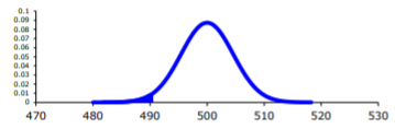
Suppose a manufacturer of the XJ35 battery claims the mean life of the battery is 500 days with a standard deviation of 25 days. You are the buyer of this battery and you think this claim is inflated. You would like to test your belief because without a good reason you can’t get out of your contract.
What do you do?
Well first, you should know what you are trying to measure. Define the random variable.
Let x = life of a XJ35 battery
Now you are not just trying to find different x values. You are trying to find what the true mean is. Since you are trying to find it, it must be unknown. You don’t think it is 500 days. If you did, you wouldn’t be doing any testing. The true mean, \(\mu\), is unknown. That means you should define that too.
Let \(\mu\)= mean life of a XJ35 battery
You may want to collect a sample. What kind of sample?
You could ask the manufacturers to give you batteries, but there is a chance that there could be some bias in the batteries they pick. To reduce the chance of bias, it is best to take a random sample.
How big should the sample be?
A sample of size 30 or more means that you can use the central limit theorem. Pick a sample of size 30.
Example \(\PageIndex{1}\) contains the data for the sample you collected:
Now what should you do? Looking at the data set, you see some of the times are above 500 and some are below. But looking at all of the numbers is too difficult. It might be helpful to calculate the mean for this sample.
The sample mean is \(\overline{x} = 490\) days. Looking at the sample mean, one might think that you are right. However, the standard deviation and the sample size also plays a role, so maybe you are wrong.
Before going any farther, it is time to formalize a few definitions.
You have a guess that the mean life of a battery is less than 500 days. This is opposed to what the manufacturer claims. There really are two hypotheses, which are just guesses here – the one that the manufacturer claims and the one that you believe. It is helpful to have names for them.
Definition \(\PageIndex{1}\)
Null Hypothesis : historical value, claim, or product specification. The symbol used is \(H_{o}\).
Definition \(\PageIndex{2}\)
Alternate Hypothesis : what you want to prove. This is what you want to accept as true when you reject the null hypothesis. There are two symbols that are commonly used for the alternative hypothesis: \(H_{A}\) or \(H_{I}\). The symbol \(H_{A}\) will be used in this book.
In general, the hypotheses look something like this:
\(H_{o} : \mu=\mu_{o}\)
\(H_{A} : \mu<\mu_{o}\)
where \(\mu_{o}\) just represents the value that the claim says the population mean is actually equal to.
Also, \(H_{A}\) can be less than, greater than, or not equal to.
For this problem:
\(H_{o} : \mu=500\) days, since the manufacturer says the mean life of a battery is 500 days.
\(H_{A} : \mu<500\) days, since you believe that the mean life of the battery is less than 500 days.
Now back to the mean. You have a sample mean of 490 days. Is this small enough to believe that you are right and the manufacturer is wrong? How small does it have to be?
If you calculated a sample mean of 235, you would definitely believe the population mean is less than 500. But even if you had a sample mean of 435 you would probably believe that the true mean was less than 500. What about 475? Or 483? There is some point where you would stop being so sure that the population mean is less than 500. That point separates the values of where you are sure or pretty sure that the mean is less than 500 from the area where you are not so sure. How do you find that point?
Well it depends on how much error you want to make. Of course you don’t want to make any errors, but unfortunately that is unavoidable in statistics. You need to figure out how much error you made with your sample. Take the sample mean, and find the probability of getting another sample mean less than it, assuming for the moment that the manufacturer is right. The idea behind this is that you want to know what is the chance that you could have come up with your sample mean even if the population mean really is 500 days.
You want to find \(P\left(\overline{x}<490 | H_{o} \text { is true }\right)=P(\overline{x}<490 | \mu=500)\)
To compute this probability, you need to know how the sample mean is distributed. Since the sample size is at least 30, then you know the sample mean is approximately normally distributed. Remember \(\mu_{\overline{x}}=\mu\) and \(\sigma_{\overline{x}}=\dfrac{\sigma}{\sqrt{n}}\)
A picture is always useful.
.png?revision=1 "hypothesis test formula statistics")
Before calculating the probability, it is useful to see how many standard deviations away from the mean the sample mean is. Using the formula for the z-score from chapter 6, you find
\(z=\dfrac{\overline{x}-\mu_{o}}{\sigma / \sqrt{n}}=\dfrac{490-500}{25 / \sqrt{30}}=-2.19\)
This sample mean is more than two standard deviations away from the mean. That seems pretty far, but you should look at the probability too.
On TI-83/84:
\(P(\overline{x}<490 | \mu=500)=\text { normalcdf }(-1 E 99,490,500,25 \div \sqrt{30}) \approx 0.0142\)
\(P(\overline{x}<490 \mu=500)=\text { pnorm }(490,500,25 / \operatorname{sqrt}(30)) \approx 0.0142\)
There is a 1.42% chance that you could find a sample mean less than 490 when the population mean is 500 days. This is really small, so the chances are that the assumption that the population mean is 500 days is wrong, and you can reject the manufacturer’s claim. But how do you quantify really small? Is 5% or 10% or 15% really small? How do you decide?
Before you answer that question, a couple more definitions are needed.
Definition \(\PageIndex{3}\)
Test Statistic : \(z=\dfrac{\overline{x}-\mu_{o}}{\sigma / \sqrt{n}}\) since it is calculated as part of the testing of the hypothesis.
Definition \(\PageIndex{4}\)
p – value : probability that the test statistic will take on more extreme values than the observed test statistic, given that the null hypothesis is true. It is the probability that was calculated above.
Now, how small is small enough? To answer that, you really want to know the types of errors you can make.
There are actually only two errors that can be made. The first error is if you say that \(H_{o}\) is false, when in fact it is true. This means you reject \(H_{o}\) when \(H_{o}\) was true. The second error is if you say that \(H_{o}\) is true, when in fact it is false. This means you fail to reject \(H_{o}\) when \(H_{o}\) is false. The following table organizes this for you:
Type of errors:
Definition \(\PageIndex{5}\)
Type I Error is rejecting \(H_{o}\) when \(H_{o}\) is true, and
Definition \(\PageIndex{6}\)
Type II Error is failing to reject \(H_{o}\) when \(H_{o}\) is false.
Since these are the errors, then one can define the probabilities attached to each error.
Definition \(\PageIndex{7}\)
\(\alpha\) = P(type I error) = P(rejecting \(H_{o} / H_{o}\) is true)
Definition \(\PageIndex{8}\)
\(\beta\) = P(type II error) = P(failing to reject \(H_{o} / H_{o}\) is false)
\(\alpha\) is also called the level of significance .
Another common concept that is used is Power = \(1-\beta \).
Now there is a relationship between \(\alpha\) and \(\beta\). They are not complements of each other. How are they related?
If \(\alpha\) increases that means the chances of making a type I error will increase. It is more likely that a type I error will occur. It makes sense that you are less likely to make type II errors, only because you will be rejecting \(H_{o}\) more often. You will be failing to reject \(H_{o}\) less, and therefore, the chance of making a type II error will decrease. Thus, as \(\alpha\) increases, \(\beta\) will decrease, and vice versa. That makes them seem like complements, but they aren’t complements. What gives? Consider one more factor – sample size.
Consider if you have a larger sample that is representative of the population, then it makes sense that you have more accuracy then with a smaller sample. Think of it this way, which would you trust more, a sample mean of 490 if you had a sample size of 35 or sample size of 350 (assuming a representative sample)? Of course the 350 because there are more data points and so more accuracy. If you are more accurate, then there is less chance that you will make any error. By increasing the sample size of a representative sample, you decrease both \(\alpha\) and \(\beta\).
Summary of all of this:
- For a certain sample size, n , if \(\alpha\) increases, \(\beta\) decreases.
- For a certain level of significance, \(\alpha\), if n increases, \(\beta\) decreases.
Now how do you find \(\alpha\) and \(\beta\)? Well \(\alpha\) is actually chosen. There are only three values that are usually picked for \(\alpha\): 0.01, 0.05, and 0.10. \(\beta\) is very difficult to find, so usually it isn’t found. If you want to make sure it is small you take as large of a sample as you can afford provided it is a representative sample. This is one use of the Power. You want \(\beta\) to be small and the Power of the test is large. The Power word sounds good.
Which pick of \(\alpha\) do you pick? Well that depends on what you are working on. Remember in this example you are the buyer who is trying to get out of a contract to buy these batteries. If you create a type I error, you said that the batteries are bad when they aren’t, most likely the manufacturer will sue you. You want to avoid this. You might pick \(\alpha\) to be 0.01. This way you have a small chance of making a type I error. Of course this means you have more of a chance of making a type II error. No big deal right? What if the batteries are used in pacemakers and you tell the person that their pacemaker’s batteries are good for 500 days when they actually last less, that might be bad. If you make a type II error, you say that the batteries do last 500 days when they last less, then you have the possibility of killing someone. You certainly do not want to do this. In this case you might want to pick \(\alpha\) as 0.10. If both errors are equally bad, then pick \(\alpha\) as 0.05.
The above discussion is why the choice of \(\alpha\) depends on what you are researching. As the researcher, you are the one that needs to decide what \(\alpha\) level to use based on your analysis of the consequences of making each error is.
If a type I error is really bad, then pick \(\alpha\) = 0.01.
If a type II error is really bad, then pick \(\alpha\) = 0.10
If neither error is bad, or both are equally bad, then pick \(\alpha\) = 0.05
The main thing is to always pick the \(\alpha\) before you collect the data and start the test.
The above discussion was long, but it is really important information. If you don’t know what the errors of the test are about, then there really is no point in making conclusions with the tests. Make sure you understand what the two errors are and what the probabilities are for them.
Now it is time to go back to the example and put this all together. This is the basic structure of testing a hypothesis, usually called a hypothesis test. Since this one has a test statistic involving z, it is also called a z-test. And since there is only one sample, it is usually called a one-sample z-test.
Example \(\PageIndex{2}\) battery example revisited
- State the random variable and the parameter in words.
- State the null and alternative hypothesis and the level of significance.
- A random sample of size n is taken.
- The population standard derivation is known.
- The sample size is at least 30 or the population of the random variable is normally distributed.
- Find the sample statistic, test statistic, and p-value.
- Interpretation
1. x = life of battery
\(\mu\) = mean life of a XJ35 battery
2. \(H_{o} : \mu=500\) days
\(H_{A} : \mu<500\) days
\(\alpha = 0.10\) (from above discussion about consequences)
3. Every hypothesis has some assumptions that be met to make sure that the results of the hypothesis are valid. The assumptions are different for each test. This test has the following assumptions.
- This occurred in this example, since it was stated that a random sample of 30 battery lives were taken.
- This is true, since it was given in the problem.
- The sample size was 30, so this condition is met.
4. The test statistic depends on how many samples there are, what parameter you are testing, and assumptions that need to be checked. In this case, there is one sample and you are testing the mean. The assumptions were checked above.
Sample statistic:
\(\overline{x} = 490\)
Test statistic:
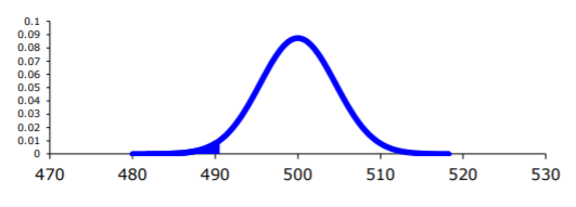.png?revision=1 "hypothesis test formula statistics")
Using TI-83/84:
\(P(\overline{x}<490 | \mu=500)=\text { normalcdf }(-1 \mathrm{E} 99,490,500,25 / \sqrt{30}) \approx 0.0142\)
\(P(\overline{x}<490 | \mu=500)=\operatorname{pnorm}(490,500,25 / \operatorname{sqrt}(30)) \approx 0.0142\)
5. Now what? Well, this p-value is 0.0142. This is a lot smaller than the amount of error you would accept in the problem -\(\alpha\) = 0.10. That means that finding a sample mean less than 490 days is unusual to happen if \(H_{o}\) is true. This should make you think that \(H_{o}\) is not true. You should reject \(H_{o}\).
In fact, in general:
Reject \(H_{o}\) if the p-value < \(\alpha\) and
Fail to reject \(H_{o}\) if the p-value \(\geq \alpha\).
6. Since you rejected \(H_{o}\), what does this mean in the real world? That is what goes in the interpretation. Since you rejected the claim by the manufacturer that the mean life of the batteries is 500 days, then you now can believe that your hypothesis was correct. In other words, there is enough evidence to show that the mean life of the battery is less than 500 days.
Now that you know that the batteries last less than 500 days, should you cancel the contract? Statistically, there is evidence that the batteries do not last as long as the manufacturer says they should. However, based on this sample there are only ten days less on average that the batteries last. There may not be practical significance in this case. Ten days do not seem like a large difference. In reality, if the batteries are used in pacemakers, then you would probably tell the patient to have the batteries replaced every year. You have a large buffer whether the batteries last 490 days or 500 days. It seems that it might not be worth it to break the contract over ten days. What if the 10 days was practically significant? Are there any other things you should consider? You might look at the business relationship with the manufacturer. You might also look at how much it would cost to find a new manufacturer. These are also questions to consider before making any changes. What this discussion should show you is that just because a hypothesis has statistical significance does not mean it has practical significance. The hypothesis test is just one part of a research process. There are other pieces that you need to consider.
That’s it. That is what a hypothesis test looks like. All hypothesis tests are done with the same six steps. Those general six steps are outlined below.
- State the random variable and the parameter in words. This is where you are defining what the unknowns are in this problem. x = random variable \(\mu\) = mean of random variable, if the parameter of interest is the mean. There are other parameters you can test, and you would use the appropriate symbol for that parameter.
- State the null and alternative hypotheses and the level of significance \(H_{o} : \mu=\mu_{o}\), where \(\mu_{o}\) is the known mean \(H_{A} : \mu<\mu_{o}\) \(H_{A} : \mu>\mu_{o}\), use the appropriate one for your problem \(H_{A} : \mu \neq \mu_{o}\) Also, state your \(\alpha\) level here.
- State and check the assumptions for a hypothesis test. Each hypothesis test has its own assumptions. They will be stated when the different hypothesis tests are discussed.
- Find the sample statistic, test statistic, and p-value. This depends on what parameter you are working with, how many samples, and the assumptions of the test. The p-value depends on your \(H_{A}\). If you are doing the \(H_{A}\) with the less than, then it is a left-tailed test, and you find the probability of being in that left tail. If you are doing the \(H_{A}\) with the greater than, then it is a right-tailed test, and you find the probability of being in the right tail. If you are doing the \(H_{A}\) with the not equal to, then you are doing a two-tail test, and you find the probability of being in both tails. Because of symmetry, you could find the probability in one tail and double this value to find the probability in both tails.
- Conclusion This is where you write reject \(H_{o}\) or fail to reject \(H_{o}\). The rule is: if the p-value < \(\alpha\), then reject \(H_{o}\). If the p-value \(\geq \alpha\), then fail to reject \(H_{o}\).
- Interpretation This is where you interpret in real world terms the conclusion to the test. The conclusion for a hypothesis test is that you either have enough evidence to show \(H_{A}\) is true, or you do not have enough evidence to show \(H_{A}\) is true.
Sorry, one more concept about the conclusion and interpretation. First, the conclusion is that you reject \(H_{o}\) or you fail to reject \(H_{o}\). Why was it said like this? It is because you never accept the null hypothesis. If you wanted to accept the null hypothesis, then why do the test in the first place? In the interpretation, you either have enough evidence to show \(H_{A}\) is true, or you do not have enough evidence to show \(H_{A}\) is true. You wouldn’t want to go to all this work and then find out you wanted to accept the claim. Why go through the trouble? You always want to show that the alternative hypothesis is true. Sometimes you can do that and sometimes you can’t. It doesn’t mean you proved the null hypothesis; it just means you can’t prove the alternative hypothesis. Here is an example to demonstrate this.
Example \(\PageIndex{3}\) conclusion in hypothesis tests
In the U.S. court system a jury trial could be set up as a hypothesis test. To really help you see how this works, let’s use OJ Simpson as an example. In the court system, a person is presumed innocent until he/she is proven guilty, and this is your null hypothesis. OJ Simpson was a football player in the 1970s. In 1994 his ex-wife and her friend were killed. OJ Simpson was accused of the crime, and in 1995 the case was tried. The prosecutors wanted to prove OJ was guilty of killing his wife and her friend, and that is the alternative hypothesis
\(H_{0}\): OJ is innocent of killing his wife and her friend
\(H_{A}\): OJ is guilty of killing his wife and her friend
In this case, a verdict of not guilty was given. That does not mean that he is innocent of this crime. It means there was not enough evidence to prove he was guilty. Many people believe that OJ was guilty of this crime, but the jury did not feel that the evidence presented was enough to show there was guilt. The verdict in a jury trial is always guilty or not guilty!
The same is true in a hypothesis test. There is either enough or not enough evidence to show that alternative hypothesis. It is not that you proved the null hypothesis true.
When identifying hypothesis, it is important to state your random variable and the appropriate parameter you want to make a decision about. If count something, then the random variable is the number of whatever you counted. The parameter is the proportion of what you counted. If the random variable is something you measured, then the parameter is the mean of what you measured. (Note: there are other parameters you can calculate, and some analysis of those will be presented in later chapters.)
Example \(\PageIndex{4}\) stating hypotheses
Identify the hypotheses necessary to test the following statements:
- The average salary of a teacher is more than $30,000.
- The proportion of students who like math is less than 10%.
- The average age of students in this class differs from 21.
a. x = salary of teacher
\(\mu\) = mean salary of teacher
The guess is that \(\mu>\$ 30,000\) and that is the alternative hypothesis.
The null hypothesis has the same parameter and number with an equal sign.
\(\begin{array}{l}{H_{0} : \mu=\$ 30,000} \\ {H_{A} : \mu>\$ 30,000}\end{array}\)
b. x = number od students who like math
p = proportion of students who like math
The guess is that p < 0.10 and that is the alternative hypothesis.
\(\begin{array}{l}{H_{0} : p=0.10} \\ {H_{A} : p<0.10}\end{array}\)
c. x = age of students in this class
\(\mu\) = mean age of students in this class
The guess is that \(\mu \neq 21\) and that is the alternative hypothesis.
\(\begin{array}{c}{H_{0} : \mu=21} \\ {H_{A} : \mu \neq 21}\end{array}\)
Example \(\PageIndex{5}\) Stating Type I and II Errors and Picking Level of Significance
- The plant-breeding department at a major university developed a new hybrid raspberry plant called YumYum Berry. Based on research data, the claim is made that from the time shoots are planted 90 days on average are required to obtain the first berry with a standard deviation of 9.2 days. A corporation that is interested in marketing the product tests 60 shoots by planting them and recording the number of days before each plant produces its first berry. The sample mean is 92.3 days. The corporation wants to know if the mean number of days is more than the 90 days claimed. State the type I and type II errors in terms of this problem, consequences of each error, and state which level of significance to use.
- A concern was raised in Australia that the percentage of deaths of Aboriginal prisoners was higher than the percent of deaths of non-indigenous prisoners, which is 0.27%. State the type I and type II errors in terms of this problem, consequences of each error, and state which level of significance to use.
a. x = time to first berry for YumYum Berry plant
\(\mu\) = mean time to first berry for YumYum Berry plant
\(\begin{array}{l}{H_{0} : \mu=90} \\ {H_{A} : \mu>90}\end{array}\)
Type I Error: If the corporation does a type I error, then they will say that the plants take longer to produce than 90 days when they don’t. They probably will not want to market the plants if they think they will take longer. They will not market them even though in reality the plants do produce in 90 days. They may have loss of future earnings, but that is all.
Type II error: The corporation do not say that the plants take longer then 90 days to produce when they do take longer. Most likely they will market the plants. The plants will take longer, and so customers might get upset and then the company would get a bad reputation. This would be really bad for the company.
Level of significance: It appears that the corporation would not want to make a type II error. Pick a 10% level of significance, \(\alpha = 0.10\).
b. x = number of Aboriginal prisoners who have died
p = proportion of Aboriginal prisoners who have died
\(\begin{array}{l}{H_{o} : p=0.27 \%} \\ {H_{A} : p>0.27 \%}\end{array}\)
Type I error: Rejecting that the proportion of Aboriginal prisoners who died was 0.27%, when in fact it was 0.27%. This would mean you would say there is a problem when there isn’t one. You could anger the Aboriginal community, and spend time and energy researching something that isn’t a problem.
Type II error: Failing to reject that the proportion of Aboriginal prisoners who died was 0.27%, when in fact it is higher than 0.27%. This would mean that you wouldn’t think there was a problem with Aboriginal prisoners dying when there really is a problem. You risk causing deaths when there could be a way to avoid them.
Level of significance: It appears that both errors may be issues in this case. You wouldn’t want to anger the Aboriginal community when there isn’t an issue, and you wouldn’t want people to die when there may be a way to stop it. It may be best to pick a 5% level of significance, \(\alpha = 0.05\).
Hypothesis testing is really easy if you follow the same recipe every time. The only differences in the various problems are the assumptions of the test and the test statistic you calculate so you can find the p-value. Do the same steps, in the same order, with the same words, every time and these problems become very easy.
Exercise \(\PageIndex{1}\)
For the problems in this section, a question is being asked. This is to help you understand what the hypotheses are. You are not to run any hypothesis tests and come up with any conclusions in this section.
- Eyeglassomatic manufactures eyeglasses for different retailers. They test to see how many defective lenses they made in a given time period and found that 11% of all lenses had defects of some type. Looking at the type of defects, they found in a three-month time period that out of 34,641 defective lenses, 5865 were due to scratches. Are there more defects from scratches than from all other causes? State the random variable, population parameter, and hypotheses.
- According to the February 2008 Federal Trade Commission report on consumer fraud and identity theft, 23% of all complaints in 2007 were for identity theft. In that year, Alaska had 321 complaints of identity theft out of 1,432 consumer complaints ("Consumer fraud and," 2008). Does this data provide enough evidence to show that Alaska had a lower proportion of identity theft than 23%? State the random variable, population parameter, and hypotheses.
- The Kyoto Protocol was signed in 1997, and required countries to start reducing their carbon emissions. The protocol became enforceable in February 2005. In 2004, the mean CO2 emission was 4.87 metric tons per capita. Is there enough evidence to show that the mean CO2 emission is lower in 2010 than in 2004? State the random variable, population parameter, and hypotheses.
- The FDA regulates that fish that is consumed is allowed to contain 1.0 mg/kg of mercury. In Florida, bass fish were collected in 53 different lakes to measure the amount of mercury in the fish. The data for the average amount of mercury in each lake is in Example \(\PageIndex{5}\) ("Multi-disciplinary niser activity," 2013). Do the data provide enough evidence to show that the fish in Florida lakes has more mercury than the allowable amount? State the random variable, population parameter, and hypotheses.
- Eyeglassomatic manufactures eyeglasses for different retailers. They test to see how many defective lenses they made in a given time period and found that 11% of all lenses had defects of some type. Looking at the type of defects, they found in a three-month time period that out of 34,641 defective lenses, 5865 were due to scratches. Are there more defects from scratches than from all other causes? State the type I and type II errors in this case, consequences of each error type for this situation from the perspective of the manufacturer, and the appropriate alpha level to use. State why you picked this alpha level.
- According to the February 2008 Federal Trade Commission report on consumer fraud and identity theft, 23% of all complaints in 2007 were for identity theft. In that year, Alaska had 321 complaints of identity theft out of 1,432 consumer complaints ("Consumer fraud and," 2008). Does this data provide enough evidence to show that Alaska had a lower proportion of identity theft than 23%? State the type I and type II errors in this case, consequences of each error type for this situation from the perspective of the state of Arizona, and the appropriate alpha level to use. State why you picked this alpha level.
- The Kyoto Protocol was signed in 1997, and required countries to start reducing their carbon emissions. The protocol became enforceable in February 2005. In 2004, the mean CO2 emission was 4.87 metric tons per capita. Is there enough evidence to show that the mean CO2 emission is lower in 2010 than in 2004? State the type I and type II errors in this case, consequences of each error type for this situation from the perspective of the agency overseeing the protocol, and the appropriate alpha level to use. State why you picked this alpha level.
- The FDA regulates that fish that is consumed is allowed to contain 1.0 mg/kg of mercury. In Florida, bass fish were collected in 53 different lakes to measure the amount of mercury in the fish. The data for the average amount of mercury in each lake is in Example \(\PageIndex{5}\) ("Multi-disciplinary niser activity," 2013). Do the data provide enough evidence to show that the fish in Florida lakes has more mercury than the allowable amount? State the type I and type II errors in this case, consequences of each error type for this situation from the perspective of the FDA, and the appropriate alpha level to use. State why you picked this alpha level.
1. \(H_{o} : p=0.11, H_{A} : p>0.11\)
3. \(H_{o} : \mu=4.87 \text { metric tons per capita, } H_{A} : \mu<4.87 \text { metric tons per capita }\)
5. See solutions
7. See solutions
IMAGES
VIDEO
COMMENTS
Table of contents. Step 1: State your null and alternate hypothesis. Step 2: Collect data. Step 3: Perform a statistical test. Step 4: Decide whether to reject or fail to reject your null hypothesis. Step 5: Present your findings. Other interesting articles. Frequently asked questions about hypothesis testing.
Test statistics represent effect sizes in hypothesis tests because they denote the difference between your sample effect and no effect —the null hypothesis. Consequently, you use the test statistic to calculate the p-value for your hypothesis test. The above p-value definition is a bit tortuous.
Hypothesis testing is a tool for making statistical inferences about the population data. It is an analysis tool that tests assumptions and determines how likely something is within a given standard of accuracy. Hypothesis testing provides a way to verify whether the results of an experiment are valid. A null hypothesis and an alternative ...
3. Find the test statistic. Find the test statistic and the corresponding p-value. Often we are analyzing a population mean or proportion and the general formula to find the test statistic is: (sample statistic – population parameter) / (standard deviation of statistic) 4. Reject or fail to reject the null hypothesis. Using the test statistic ...
This page titled 9.1: Introduction to Hypothesis Testing is shared under a CC BY 2.0 license and was authored, remixed, and/or curated by Kyle Siegrist ( Random Services) via source content that was edited to the style and standards of the LibreTexts platform; a detailed edit history is available upon request. In hypothesis testing, the goal is ...
Below these are summarized into six such steps to conducting a test of a hypothesis. Set up the hypotheses and check conditions: Each hypothesis test includes two hypotheses about the population. One is the null hypothesis, notated as H 0, which is a statement of a particular parameter value. This hypothesis is assumed to be true until there is ...
An area of .05 is equal to a z-score of 1.645. Step 6: Find the test statistic using this formula: For this set of data: z= (112.5 – 100) / (15/√30) = 4.56. Step 6: If Step 6 is greater than Step 5, reject the null hypothesis. If it’s less than Step 5, you cannot reject the null hypothesis.
Unit test. Significance tests give us a formal process for using sample data to evaluate the likelihood of some claim about a population value. Learn how to conduct significance tests and calculate p-values to see how likely a sample result is to occur by random chance. You'll also see how we use p-values to make conclusions about hypotheses.
A statistical hypothesis test typically involves a calculation of a test statistic. Then a decision is made, either by comparing the test statistic to a critical value or equivalently by evaluating a p-value computed from the test statistic. Roughly 100 specialized statistical tests have been defined.
Test Statistic: z = x¯¯¯ −μo σ/ n−−√ z = x ¯ − μ o σ / n since it is calculated as part of the testing of the hypothesis. Definition 7.1.4 7.1. 4. p – value: probability that the test statistic will take on more extreme values than the observed test statistic, given that the null hypothesis is true.